2 Solving the inference bottleneck with the key-value cache

This chapter covers

• The inefficiency of autoregressive LLM inference
• The Key-Value Cache: a solution with a cost
• MQA and GQA: First-Gen Solutions to KV Cache Memory Limits

To understand the key innovations in the DeepSeek architecture, we must begin with the technical problem they were designed to address. Our journey follows the four-stage roadmap outlined at the start of this book, and this chapter is dedicated entirely to Stage 1: The Key-Value Cache Foundation. This stage addresses the most fundamental bottleneck in modern LLM inference. Before we can appreciate advanced architectural choices like DeepSeek’s Multi-Head Latent Attention (MLA) in Stage 2, we must first master the mechanisms it evolved from and the problems it was designed to solve.

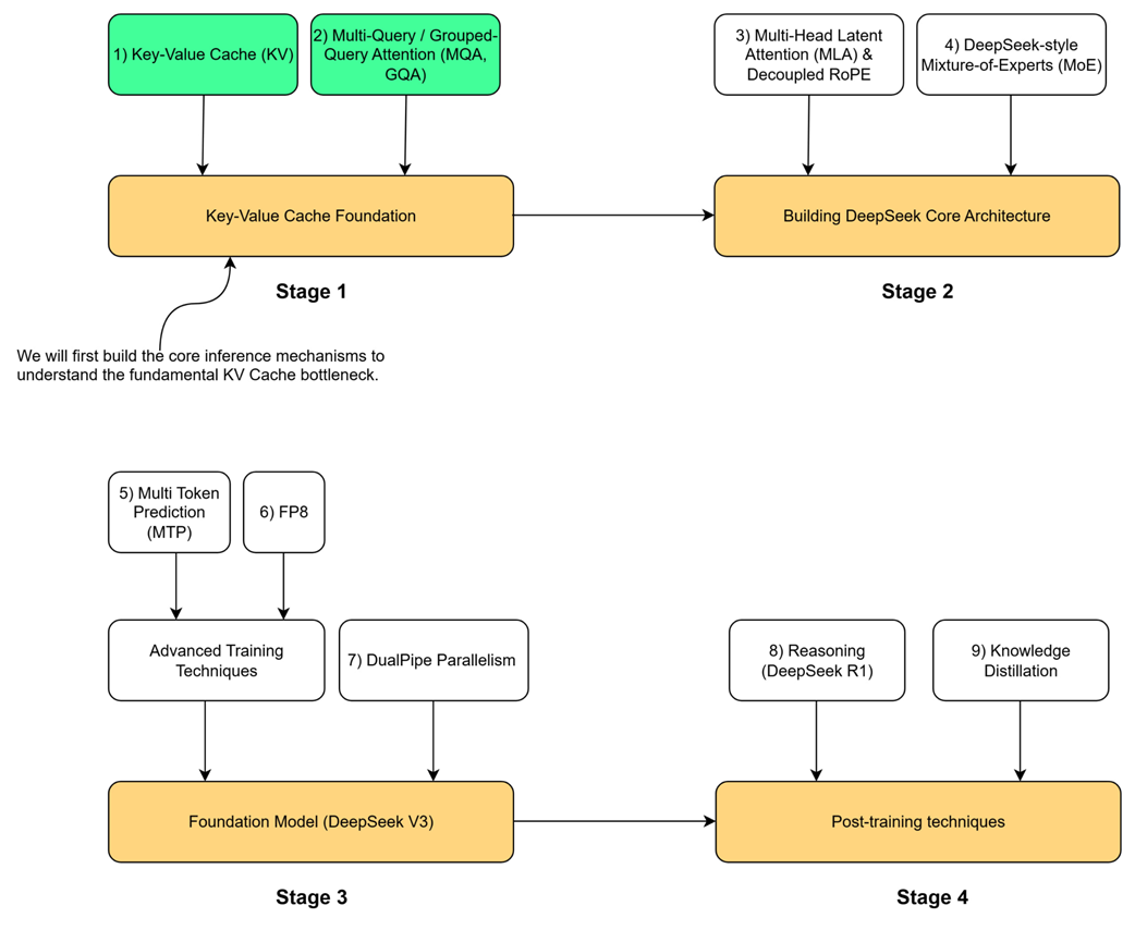
As the roadmap shows, this foundation is built on two core concepts: the Key-Value (KV) Cache itself and its first-generation optimizations, Multi-Query and Grouped-Query Attention (MQA & GQA). These techniques form the bedrock upon which more advanced architectures are built. Stage 2 of our roadmap introduces the core architectural innovations from DeepSeek-V2: Multi-Head Latent Attention (MLA), Decoupled RoPE and DeepSeek- Mixture-of-Experts (MoE). Before we can tackle those, we must first build a foundational understanding of the problems they were designed to solve. This chapter is divided into three parts to build this foundational understanding from the ground up:

First, we will build a complete autoregressive generation loop, visualizing how language models generate text one token at a time. This hands-on implementation will allow us to witness firsthand the computational inefficiencies of the traditional approach.

Second, we will implement the KV Cache itself, the elegant optimization that solves this initial performance problem. Through our code, we will demonstrate its dramatic speedup, but also uncover its “dark side”: a massive memory cost that creates a new, severe bottleneck.

Finally, we will build functional PyTorch layers for Multi-Query Attention (MQA) and Grouped-Query Attention (GQA). These are the first-generation architectural solutions designed to mitigate the KV Cache’s memory problem. It’s important to understand that these solutions are not a free lunch; both MQA and GQA explicitly trade off model quality and expressivity for gains in memory efficiency and inference speed. MQA represents an extreme on this spectrum, prioritizing memory savings above all, while GQA offers a more balanced compromise. By constructing these industry-standard techniques and understanding their inherent trade-offs, we will have the complete context needed to tackle DeepSeek’s unique innovations, which aim to achieve the best of both worlds, in the chapters to come.

2.1 The LLM inference loop: Generating text one token at a time

The first and most important concept to grasp is that the KV cache is only relevant during the inference stage of a language model. This distinction is critical, so let’s clarify the two main phases of an LLM’s life.

2.1.1 Distinguishing pre-training from inference

Every large language model, from GPT-2 to DeepSeek-V3, goes through two distinct phases:

1. Training: This is the massive, computationally expensive learning phase. The model is trained on a vast dataset (trillions of tokens) to learn grammar, facts, reasoning patterns, and the statistical relationships between words. During this phase, its parameters (or weights) are adjusted. Once pre-training is complete, the model’s parameters are fixed, resulting in a pre-trained LLM.
2. Inference: This is the “usage” phase. The pre-trained model, with its fixed parameters, is now used to perform tasks. When you interact with ChatGPT or use an API to ask a model to “make a travel plan for Italy,” you are performing inference. The model isn’t learning anymore; it’s using its learned knowledge to predict the next token in a sequence.

The entire discussion in this chapter applies exclusively to the inference stage. We assume we have a fully trained model, and our goal is simply to use it to generate text.

2.1.2 The autoregressive process: Appending tokens to build context

During inference, a language model generates text one token at a time. While a user interface like ChatGPT might make it look like the entire response appears at once, underneath the hood, a methodical, step-by-step process is unfolding. This is called autoregressive generation.

The core idea is simple but powerful: each new token the model generates is immediately added back to the input sequence, becoming part of the context for generating the next token. This creates a feedback loop that allows the model to build coherent and contextually relevant text.

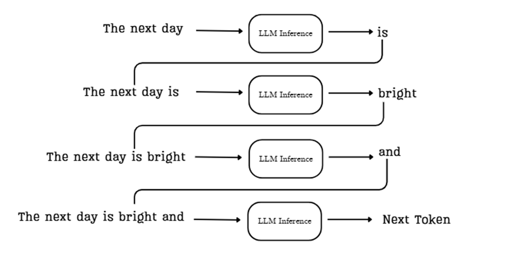
Let’s trace the flow shown in the diagram:

Sidebar “The next day.”.

The model’s task is to predict the most likely token to follow this sequence. Here’s how the process works:

1. Initial Context: We start by providing the model with an initial prompt, such as “The next day.”
2. First Prediction: This sequence is fed into the LLM inference pipeline, which processes the context and predicts the most probable next token, in this case, “is.”
3. Append and Repeat: The new token, “is,” is appended to the sequence. The input for the next step is now the expanded context: “The next day is.” This new, longer sequence is fed back into the model.
4. Second Prediction: The model now processes “The next day is” and predicts the next token, “bright.” This process continues, with the context growing one token at a time.

This loop continues, with each newly generated token being added back to the input sequence for the next prediction step. The process stops when the model generates a special end-of-sequence token or reaches a predefined limit on the number of new tokens to generate.

This iterative, feedback-driven process is fundamental to how autoregressive LLMs like the transformer construct coherent and contextually relevant text. Keep this flow in mind, as it’s the key to understanding why the KV cache is both necessary and problematic within this architectural paradigm.

2.1.3 Visualizing autoregressive generation with GPT-2

The following listing demonstrates the autoregressive loop in action using the pre-trained GPT-2 model. The code starts with an initial prompt and then enters a loop. Inside this loop, it performs the core task: it passes the current sequence to the model, gets the prediction for the very next token, and immediately appends that new token to the sequence for the next iteration. This simple visualization makes it clear that the model is performing a full computational pass for every single new token it generates.

You can find this code, along with other code listings in this book, in the official GitHub repository: https://github.com/VizuaraAI/DeepSeek-From-Scratch.

Listing 2.1 Visualizing autoregressive generation with GPT-2

from transformers import GPT2LMHeadModel, GPT2Tokenizer
import torch
 
tokenizer = GPT2Tokenizer.from_pretrained("gpt2")
model = GPT2LMHeadModel.from_pretrained("gpt2")
 
prompt = "The next day is bright"
inputs = tokenizer(prompt, return_tensors="pt")
input_ids = inputs.input_ids
 
print(f"Prompt: '{prompt}'", end="")
 
for _ in range(20):
    # The model processes the entire current sequence of tokens on every pass.
    outputs = model(input_ids)
    logits = outputs.logits
 
    # We only use the logits from the very last token to predict the next one.
    next_token_logits = logits[:, -1, :]
    next_token_id = next_token_logits.argmax(dim=-1).unsqueeze(-1)
 
    # The newly predicted token is appended to the input sequence, 
    # which is then fed back into the model in the next loop. 
    # This is the core of the autoregressive process.
    input_ids = torch.cat([input_ids, next_token_id], dim=-1)
 
    new_token = tokenizer.decode(next_token_id[0])
    print(new_token, end="", flush=True)
 
print("\n")

Running this code produces the following output, where the text after the initial prompt is generated token by token:

‘The next day is bright and sunny, and the sun is shining. The sun is shining, and the moon is shining.

This simple demonstration makes a crucial point clear: the model is performing a full computational pass through its architecture for every single new token it generates.

This is evident because the call to outputs = model(input_ids) happens inside the for loop, and the input_ids tensor, which contains the entire sequence so far, is passed to the model on every single iteration. This observation leads us to a critical question: what exactly is happening inside that computation, and is all of it truly necessary?

2.2 The core task: Predicting the next token

Now we know that the LLM performs a full computational pass for each new token. Let’s peel back the layers of the architecture to understand what that computation entails. Let’s focus on the heart of the Transformer block: the Multi-Head Attention mechanism. This is where the model figures out the relationships between tokens.

The diagram below provides a high-level map of this journey. It shows how our example, “The next day is bright,” flows through the key components we will deconstruct in the coming sections. Keep this image in mind as it represents the entire process we are about to build.

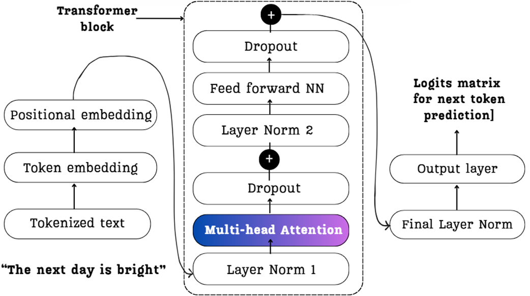
2.2.1 From input embeddings to context vectors: A mathematical walkthrough

The diagram in Figure 2.3 showed us the major components, but to understand the computations we might be repeating during inference, we need to zoom in on the most critical component: the Multi-Head Attention block. This is where the model calculates the relationships between tokens and creates the enriched “context vectors” that form the basis of its understanding.

Let’s trace the path of our input sequence, “The next day is,” through a single attention calculation to see exactly what’s happening under the hood.

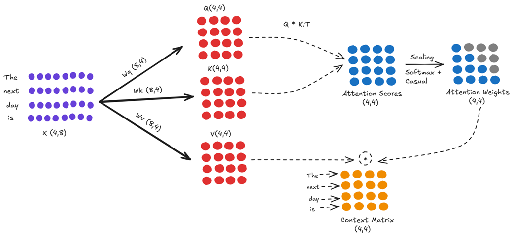
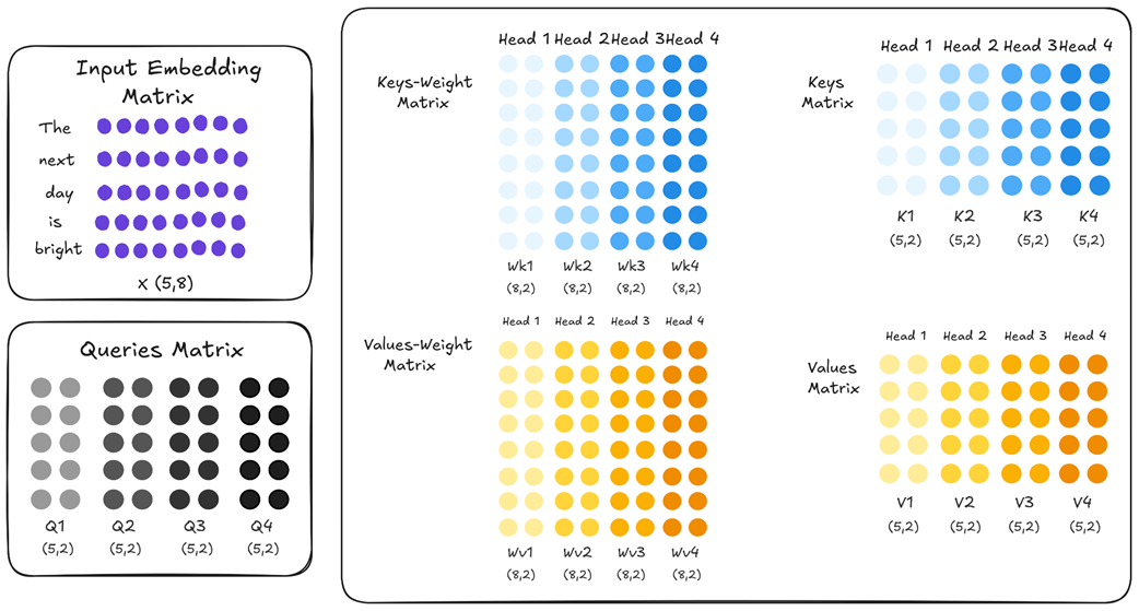
Step 1: Projecting Inputs into Query, Key, and Value

After tokenization and embedding, our input is represented as a matrix, which we’ll call X. For this walkthrough, we will use small, simplified dimensions to make the mathematics and diagrams easy to follow. Let’s assume our matrix X has a shape of (4, 8), representing our four tokens, each with an 8-dimensional embedding. In a real model, this embedding dimension would be much larger, for example, 5120 in DeepSeek-V2 and 7168 in DeepSeek-V3, but the underlying mathematical principles remain identical.

The very first step within the attention block is to project this input matrix into three distinct representations: the Query (Q), Key (K), and Value (V) matrices. This is done by multiplying X with three separate, learnable weight matrices: Wq (for Query), Wk (for Key), and Wv (for Value).

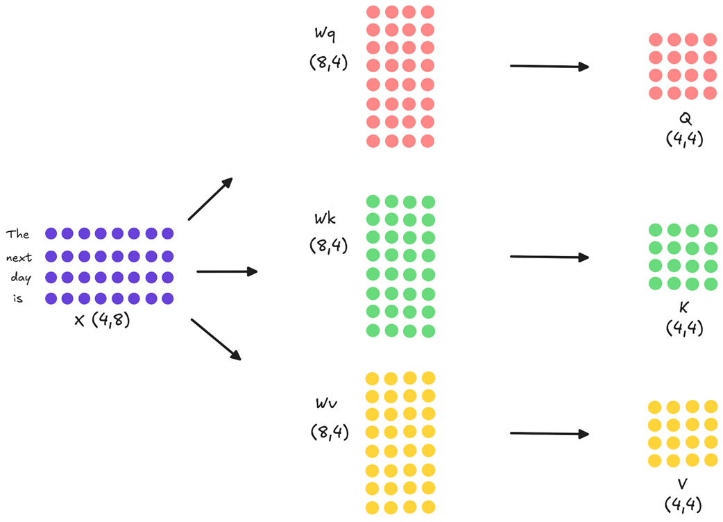
As the diagram illustrates:

• The input X (shape 4x8) is multiplied by Wq (shape 8x4) to produce the Query matrix (shape 4x4).
• The input X (shape 4x8) is multiplied by Wk (shape 8x4) to produce the Key matrix (shape 4x4).
• The input X (shape 4x8) is multiplied by Wv (shape 8x4) to produce the Value matrix (shape 4x4).

These three new matrices represent our input tokens in different roles. The Query matrix represents what each token is “looking for,” while the Key and Value matrices represent what each token “offers” as context.

Step 2: Calculating Attention Scores

Next, the model needs to determine how relevant each token is to every other token. This is done by calculating attention scores. We take the Query matrix and perform a matrix multiplication with the transpose of the Key matrix (Q * K.T).

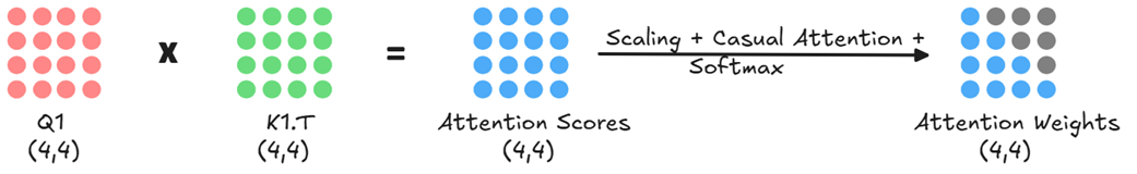
The resulting Attention Scores matrix (shape 4x4) quantifies the relationship between every pair of tokens. For example, the value in the fourth row and second column would represent how much attention the token “is” should pay to the token “next.”

Step 3: From Scores to Context Vectors

These raw scores are then processed further. They are scaled (to stabilize training), and a causal mask is applied to ensure tokens can only gather context from previous tokens in the sequence, preventing it from “cheating” by looking ahead at tokens it is not supposed to know about yet. This mask effectively zeroes out the upper triangle of the attention scores matrix. Finally, a softmax function is applied to convert the scores into attention weights, a set of probabilities that sum to 1 for each row.

These final attention weights are then multiplied by the Value matrix.

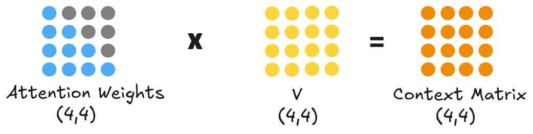
This final multiplication produces the Context Matrix (shape 4x4). Each row in this matrix is a new, enriched vector for each of our input tokens. The context vector for “is,” for example, is now a weighted sum of all the Value vectors that came before it, containing rich information about the entire preceding sequence.

Step 4: Scaling to Multi-Head Attention

The process we’ve just described above is for a single attention calculation. However, a model might need to track different kinds of relationships simultaneously; for example, syntactic dependencies (like subject-verb agreement) and semantic relationships (like word meanings). A single attention calculation might struggle to capture this diversity.

This is where multi-head attention comes in. Instead of one large set of projection matrices (Wq, Wk, Wv), the model uses multiple, smaller, independent sets - one for each “head.”

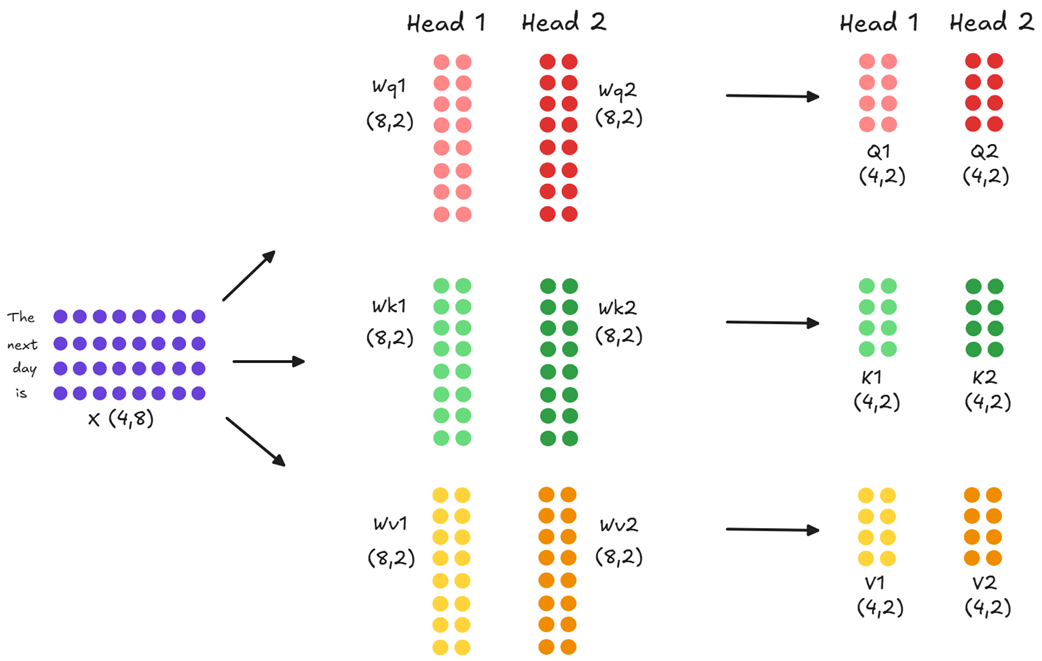
As shown in figure 2.7, if our model has two heads, the initial (4, 8) input embedding is not projected into three (4, 4) matrices. Instead, it is projected in parallel into six smaller (4, 2) matrices: Q1, K1, V1 for Head 1, and Q2, K2, V2 for Head 2.

Next, each head computes its own attention scores independently and in parallel. Head 1 calculates the relevance between its queries (Q1) and keys (K1), while Head 2 does the same with Q2 and K2.

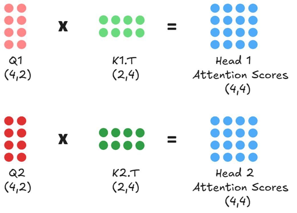
This ability to analyze the input from multiple perspectives simultaneously is the core of multi-head attention’s power. By having its own unique projection matrices, each head learns to view the input in a different representational subspace. This allows for specialization: Head 1 might learn to focus on grammatical structure, while Head 2 might focus on semantic meaning, all from the same input sequence.

After each head has independently calculated its raw attention scores, these scores represent a measure of raw, unnormalized relevance. For Head 1, its (4, 4) Attention Scores matrix tells it how strongly each of its queries connects with each of its keys. However, these raw scores are not yet in a usable format for creating a weighted average. To make them useful, each head processes its score matrix through a series of transformations, as shown in figure 2.9.

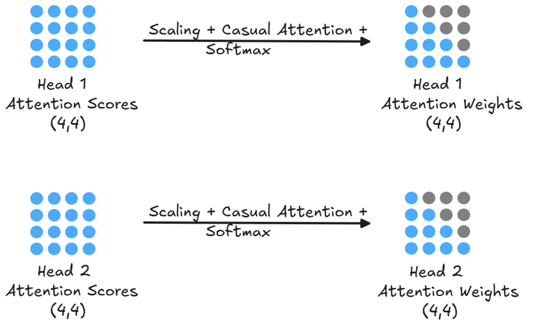
Just like in the single-head case, each head’s raw attention scores are then scaled, masked, and converted into a probability distribution of attention weights via a softmax function.

With the final, normalized attention weights for each head, the model can now create its enriched output. This is achieved by multiplying each head’s Attention Weights matrix with its corresponding Value matrix.

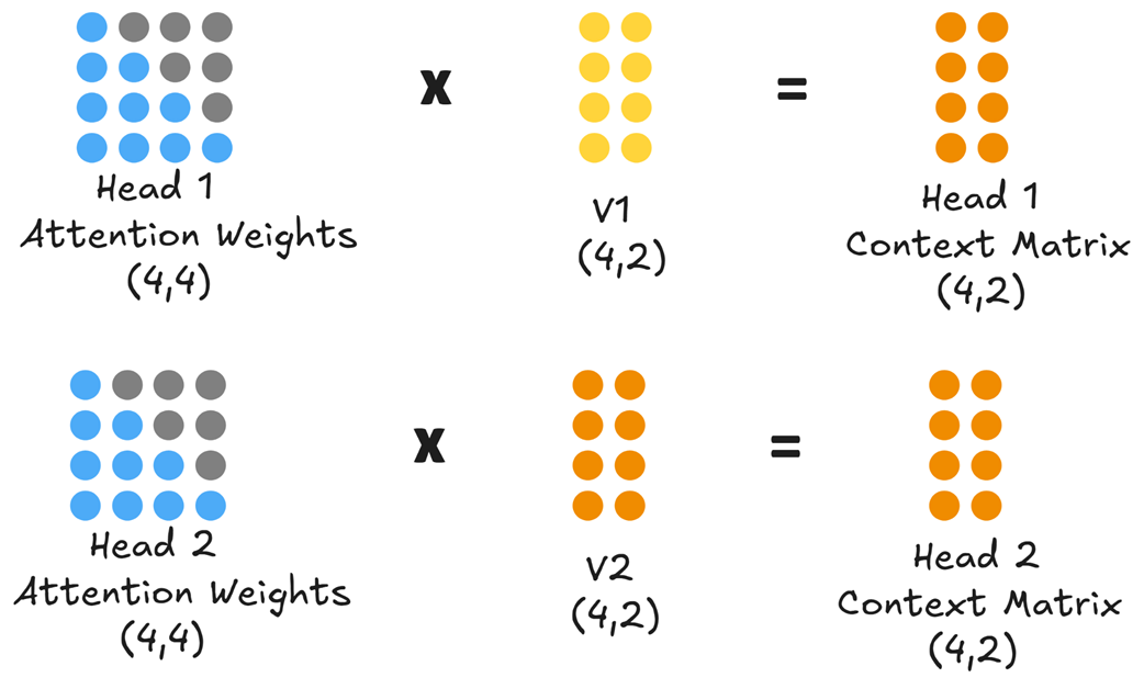
At the end of this step, we have two separate context matrices: Head 1 Context Matrix and Head 2 Context Matrix, both of shape (4, 2). Each matrix is a different contextualized representation of the original input. The final step in the multi-head attention block is to unify these parallel streams of information back into a single representation that the next layer can use. This is done in two stages.

First, the individual context matrices from all the heads are concatenated together along their last dimension (column-wise).

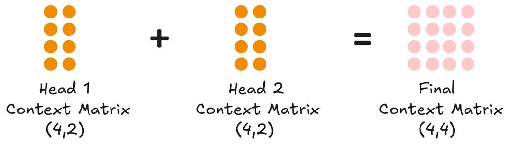
As shown in figure 2.11, concatenating the Head 1 Context Matrix (shape 4, 2) and the Head 2 Context Matrix (shape 4, 2) results in a combined matrix of shape (4, 4). This new matrix now contains the insights from both heads.

Second, this concatenated matrix is passed through one final linear layer, often called the output projection layer. This layer has its own learnable weights and is responsible for mixing the information from the different heads and projecting it back into the main model’s expected dimension, producing the final Context Matrix (shape 4, 4) that exits the multi-head attention block.

This parallel, multi-faceted, and finally unified approach is what gives the Transformer architecture its expressive power. The Context Matrix it produces is what gets passed to the subsequent layers to eventually produce the logits for our next-token prediction.

2.2.2 From context vectors to logits

We saw how the attention mechanism processes our input embeddings and produces an enriched Context Matrix. For our input “The next day is,” this is a (4, 4) matrix where each row is a new, context-aware vector for each token.

It is the culmination of the model’s effort to understand the relationships between words in the sequence. Now, this matrix gets passed to the subsequent layers in the Transformer block to eventually produce the logits for our next-token prediction.

Step 1: The Feed-Forward Network

The Context Matrix first passes through a Feed-Forward Network (FFN) within the Transformer block. Unlike the attention mechanism, which looks across all tokens, the FFN processes each token’s context vector independently. It typically consists of two linear layers with a non-linear activation function in between. This step allows the model to perform more complex calculations on each token’s contextualized representation. Crucially, the FFN is designed to output a matrix of the exact same shape as its input, preserving the dimensions of our Context Matrix.

Step 2: Iterating Through the Transformer Blocks

The output from the FFN doesn’t immediately exit the model. It first goes through the final components of the current Transformer block, which include another Layer Normalization and a residual connection that adds the block’s input to its output. This entire process—attention, feed-forward network, normalization, and residual connections—constitutes one full Transformer block. The resulting matrix is then fed as the input to the next Transformer block. This cycle repeats for every block in the model’s architecture (e.g., 12 times for GPT-2 small).

Step 3: The Final Projection to Logits

After the sequence has been processed by the very last Transformer block in the stack, the resulting matrix of context vectors goes through one final Layer Normalization. This normalized matrix is then passed to the Final Output Layer, which is where the model makes its prediction.

The Output Layer performs the crucial step of projecting our context vectors into the vast space of the model’s vocabulary. Let’s define a key term: logits.

Definition

What are Logits? A logit is a raw, unnormalized score. For any given position in a sequence, the model produces a logit for every single word in its vocabulary. A higher logit score for a particular word indicates a higher likelihood that that word is the correct next token.

The Output Layer is a simple linear layer whose job is to take the final Context Matrix and transform it into the Logits Matrix.

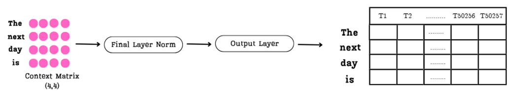
As shown in figure 2.12, the entire Context Matrix is processed. Each of its rows is transformed into a very long vector of logits:

• Input: The final Context Matrix from the last Transformer block, with shape (4, 4).
• Transformation: The Output Layer projects each of the 4 rows into a vector of size 50,257 (the vocabulary size of GPT-2).
• Output: The final Logits Matrix with shape (4, 50257).

Each row in this massive matrix represents a complete prediction. The first row contains the model’s scores for what token should follow “The,” the second row for what token should follow “next,” and so on.

Now that we have this matrix of raw scores, how does the model make a final, single-token decision? This next step contains the most important insight for optimizing the entire inference process.

2.2.3 The key insight: Why only the last row matters

We now have our Logits Matrix, a massive tensor of shape (4, 50257) containing predictions for every position in our input sequence. However, our goal is very specific: we only want to predict the single token that comes after our complete input, “The next day is.”

This means we can discard almost all of the information in the Logits Matrix.

• The first row (predictions for what comes after “The”) is irrelevant.
• The second row (predictions for what comes after “next”) is irrelevant.
• The third row (predictions for what comes after “day”) is irrelevant.

The only row we care about is the last one, the logits vector corresponding to the token “is.” This single vector holds the key to our next token. This is the crucial insight: since we only ever use the last row to make our prediction, re-computing the logits for all the earlier rows at every single step is incredibly wasteful. This observation is the fundamental motivation for optimizations like the KV cache and its derivatives, MQA and GQA.

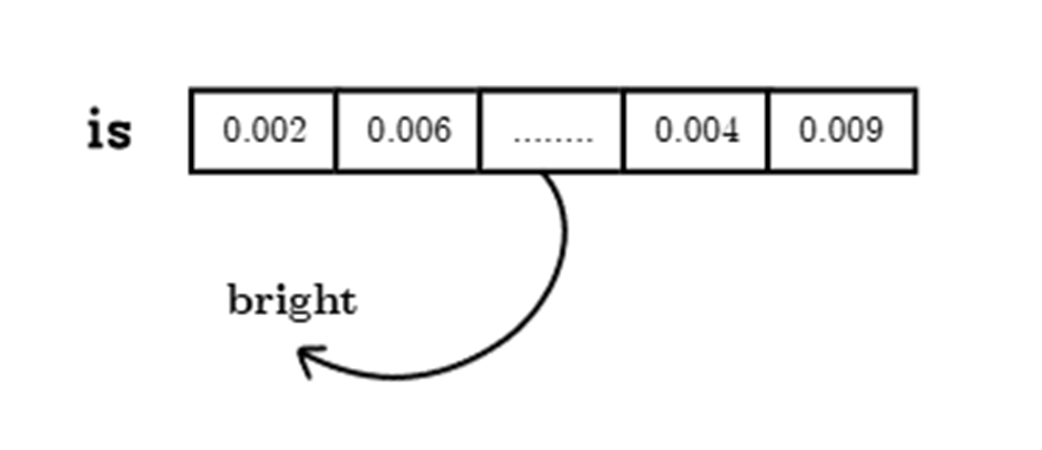
To select the next token for our input we:

• Isolate the Final Logits Vector: We select only the last row from the Logits Matrix. This gives us a vector of shape (1, 50257) containing the model’s unnormalized confidence scores for every possible word in its vocabulary.
• Apply the Softmax Function: These raw logits are converted into probabilities using the softmax function. This function transforms the entire vector into a probability distribution, where each value is between 0 and 1, and all values sum to 1. The output is a vector of probabilities, as shown in the figure with values like 0.002, 0.006, etc.
• Select the Most Likely Token: We now simply find the index of the highest probability in this distribution (an argmax operation). This index corresponds to a specific token in the model’s vocabulary. As the diagram shows, if the highest probability points to the token “bright,” then that becomes the model’s final, generated output for this step.

This entire, multi-step path from raw text to a single predicted token is performed for every token the model generates. And this gives us a key insight: after all the complex, context-building work, the final prediction depends only on the context vector of the last token. It’s crucial to remember that this last context vector is significant because, thanks to the self-attention mechanism, it already contains a weighted summary of information from all previous tokens in the sequence.

This should make you suspicious. If we are constantly feeding a growing sequence back into the model, are we doing a lot of unnecessary, repeated work in the attention block itself? As we’ll prove mathematically in the next section, the answer is a resounding yes.

2.3 The problem of redundant computations

So far, we’ve established two critical facts about LLM inference:

1. The model generates text one token at a time in an autoregressive loop, feeding its own output back as input.
2. To predict the single next token, the model only requires the context vector of the last token in the current sequence.

Now, let’s connect these two ideas. If the model is constantly re-processing a growing sequence of tokens, and it only needs the information from the very last one to make its next decision, it seems that a huge number of computations might be performed unnecessarily. Intuitively, it feels like we might be performing the same calculations again and again.

I’m going to show you that during inference, we are indeed repeating many computations. We will then see what we can do to avoid these repetitions, which will lead us directly to the concept of the KV Cache.

2.3.1 Intuition: Are we calculating the same thing over and over?

Let’s move from intuition to concrete mathematical proof. We’ll first show the redundancy intuitively by tracing the data at each step, and then we will quantify its performance impact by analyzing the computational complexity. Let’s revisit the autoregressive loop from figure 2.2, but this time, let’s focus on the data being passed into the model at each step.

Imagine we start with the prompt “The next day.”

Inference Step 1:

• Input: “The next day”
• Process: The three tokens go through the entire LLM pipeline.
• Output: “is”

Inference Step 2:

The new token is appended.

• Input: “The next day is”
• Process: These four tokens go through the entire LLM pipeline.
• Output: “bright”

Inference Step 3:

The new token is appended again.

• Input: “The next day is bright”
• Process: These five tokens go through the entire LLM pipeline.
• Output: “and”

Notice the pattern. In Step 2, we are re-processing the tokens “The,” “next,” and “day.” We already processed them in Step 1. In Step 3, we are re-processing “The,” “next,” “day,” and “is,” all of which have been processed in previous steps. It seems we are passing the same tokens through the entire architecture again and again, just to add one new token at the end.

This process feels inefficient. It’s like re-reading the first nine chapters of a book every time you want to read a new chapter. If reading each chapter takes a fixed amount of time, then reading up to chapter n requires 1 + 2 + … + n units of work—scaling quadratically, O(n²).

The main drawback of these repeated computations is their explosive cost: for every additional token, the GPU must re-process and store increasingly large amounts of data, making both time and memory requirements grow rapidly with sequence length.

This intuitive sense of repetition is, in fact, correct. Let’s take a hands-on example and prove mathematically that we are repeating the exact same calculations within the attention mechanism at every single step of inference.

2.3.2 A mathematical proof: Visualizing repeated calculations

Our intuition suggests we are performing redundant work. Now, let’s prove it by walking through the attention mechanism for two consecutive inference steps. We will see with our own eyes that we are calculating the exact same values multiple times.

Step A: Inference at Time T=4 (Input: “The next day is”)

First, let’s consider the state of our model at the moment it has processed the input “The next day is” and is about to predict the next token. This is an input sequence with 4 tokens. As shown in figure 2.14, this sequence is about to be processed by a single attention head.

Let’s trace the data flow in figure 2.14 step-by-step:

1. Input Embedding (X): We start on the far left with our input embedding matrix X, which has a shape of (4, 8) for our four tokens.
2. Projection: This X matrix is multiplied by the fixed, pre-trained weight matrices Wq, Wk, and Wv. This projection creates the Query (Q), Key (K), and Value (V) matrices, which in this example all have the shape (4, 4).
3. Attention Scores: Next, the model calculates the raw relevance between tokens. The Query matrix is multiplied by the transpose of the Key matrix (Q * K.T), resulting in the (4, 4) Attention Scores matrix.
4. Attention Weights: This raw score matrix is then processed (scaled and passed through a causal softmax) to produce the final (4, 4) Attention Weights matrix. The grayed-out parts represent future positions that have been masked to zero.
5. Context Matrix: Finally, the Attention Weights are multiplied by the Value matrix to produce the (4, 4) Context Matrix.

This Context Matrix then travels through the rest of the Transformer architecture. As we established, only the last row of this matrix—the context vector for “is”—is used to generate the final logits and predict the next token. Let’s say the model correctly predicts the token “bright.”

Now, we move to the next step in the autoregressive loop, and this is where the inefficiency becomes glaringly obvious.

Step B: Inference at Time T=5 (Input: “The next day is bright”)

Following the autoregressive loop, the newly predicted token, “bright,” is appended to our sequence. The new input for the model is now “The next day is bright,” a sequence of 5 tokens. This new, longer sequence is fed back into the exact same attention mechanism, with the exact same learned weight matrices (Wq, Wk, Wv).

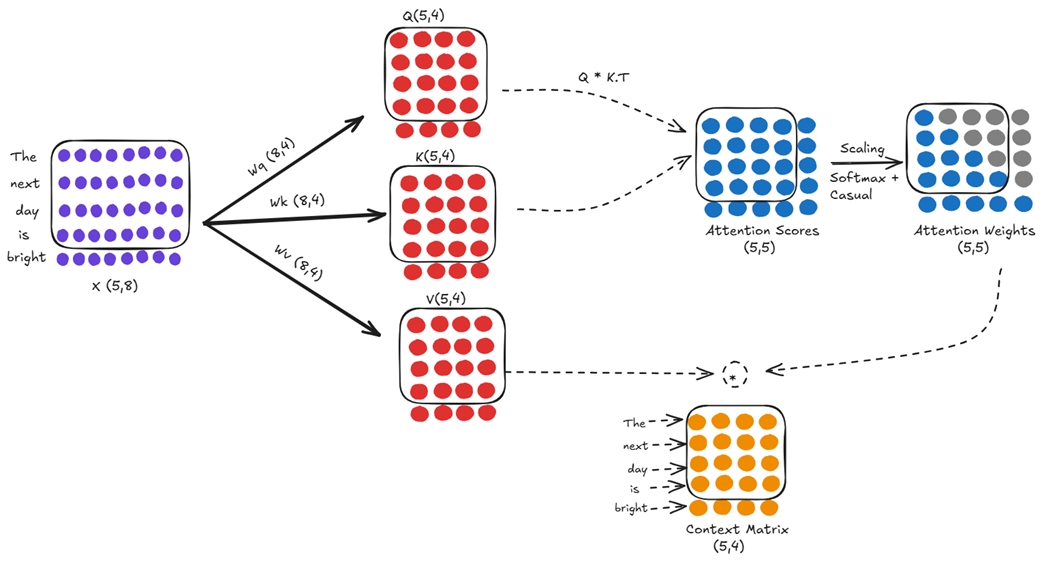
At first glance, this looks like a completely new calculation. But let’s compare it closely to the computation we just performed in figure 2.15.

The first four rows of our new input matrix X (shape 5, 8) are identical to the entire input matrix from the previous step. Since the weight matrices (Wq, Wk, Wv) are fixed during inference, this means the first four rows of our new Query, Key, and Value matrices (all now shape 5, 4) are identical to the entire Query, Key, and Value matrices from the previous step.

This redundancy cascades directly into the attention score calculation. The score at any position (j, i) is the dot product of the j-th query vector and the i-th key vector. Since the first four query vectors and the first four key vectors are identical to the previous step, the entire top-left (4, 4) sub-block of our new (5, 5) Attention Scores matrix is also identical to the entire score matrix we calculated just a moment ago.

We are performing a massive amount of redundant computation. We are re-calculating the projections and the attention scores for the entire history of the sequence at every single step. This is a huge waste of computational resources. And the most inefficient part? As we’ve established, after all this redundant work, the only piece of information we are actually going to use to predict the next token is the context vector derived from the new token, “bright.”

We are re-calculating an entire history of interactions just to compute one new row, and then we throw away most of the old row’s final outputs anyway. This is the root problem that inference optimization techniques must solve.

2.3.3 The performance impact: From quadratic to linear complexity

The redundant calculations we’ve identified are not just theoretically inefficient; they have a severe impact on performance, especially as the input sequence grows longer. This impact is best understood through the lens of computational complexity.

Note

It is important to clarify that this discussion is strictly about the inference stage.

Without any optimization, the core of the attention mechanism is quadratic in nature. For each layer and for each attention head, the number of calculations needed to compute the attention scores scales quadratically with the length of the input sequence (n), often denoted as O(n²). While the total number of computations is multiplied by constants like the number of layers (L) and heads (H), it’s the quadratic relationship with the sequence length n that dominates performance.

Why quadratic? Think about the Attention Scores matrix.

• For an input of 4 tokens, we compute a 4x4 matrix (16 scores).
• For an input of 5 tokens, we compute a 5x5 matrix (25 scores).
• For an input of 1,000 tokens, we would compute a 1,000 x 1,000 matrix (1,000,000 scores).

At each step of autoregressive generation, we are re-calculating this entire n x n matrix, performing O(n²) work repeatedly. As the sequence length n grows, the number of computations explodes. This quadratic complexity is the primary reason why unoptimized inference for long sequences is computationally expensive and extremely slow. Each new token becomes progressively slower to generate than the last because the model has to do more and more historical re-calculation.

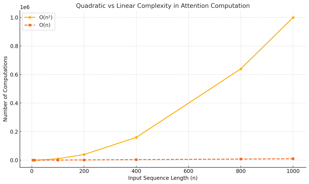
The goal of inference optimization is to transform this quadratic process into a linear one (O(n)). In a linear complexity scenario, the amount of computation required to generate a new token grows linearly with the length of the sequence, not quadratically. This means that while generating a new token for a long sequence still requires more computation than for a short one, the increase is far more manageable. For instance, doubling the context length would roughly double the work for the next token, rather than quadrupling it, preventing the explosive growth of the unoptimized approach.

This is precisely what caching allows us to achieve. By storing the results of past computations instead of repeating them, we can break free from the quadratic trap. As we saw visually, the only new computations we need to perform for a new token are related to that token itself. The computations for all previous tokens can be retrieved from memory.

This shift from quadratic to linear complexity is the fundamental reason why caching is not just an optimization but a foundational requirement for making LLMs with large context windows practical. It explains the dramatic speedups we will demonstrate in code:

• Without Caching (Quadratic): Generating the 100th token is much slower than generating the 10th token.
• With Caching (Linear): Generating the 100th token takes roughly the same amount of time as generating the 10th token.

Having established the dire need for a solution, we are now ready to build it.

2.4 The solution: Caching for efficiency

The solution to this problem is both elegant and intuitive: if we are repeatedly calculating the same values, why not just calculate them once and store them for future use? This is the core principle of caching.

By storing the results of past computations, we can avoid re-doing the work for tokens we’ve already seen. This allows us to break free from the quadratic trap and achieve a much more efficient, linear computation time. This powerful optimization is known as the Key-Value Cache, or KV Cache.

2.4.1 What to cache? A step-by-step derivation

To understand what we need to cache, we must start with our end goal and work backward. As we established in section 2.2.3, our entire objective at each inference step is to produce the single context vector for the most recent token.

Let’s take our example where the model has just processed “The next day is” and generated “bright.” The new input sequence is now 5 tokens long. To predict the next token, we only need the context vector for “bright.”

The values shown in the box are from previous steps. Since these values remain unchanged across steps, we cache them. The same principle applies to the subsequent images in this section.

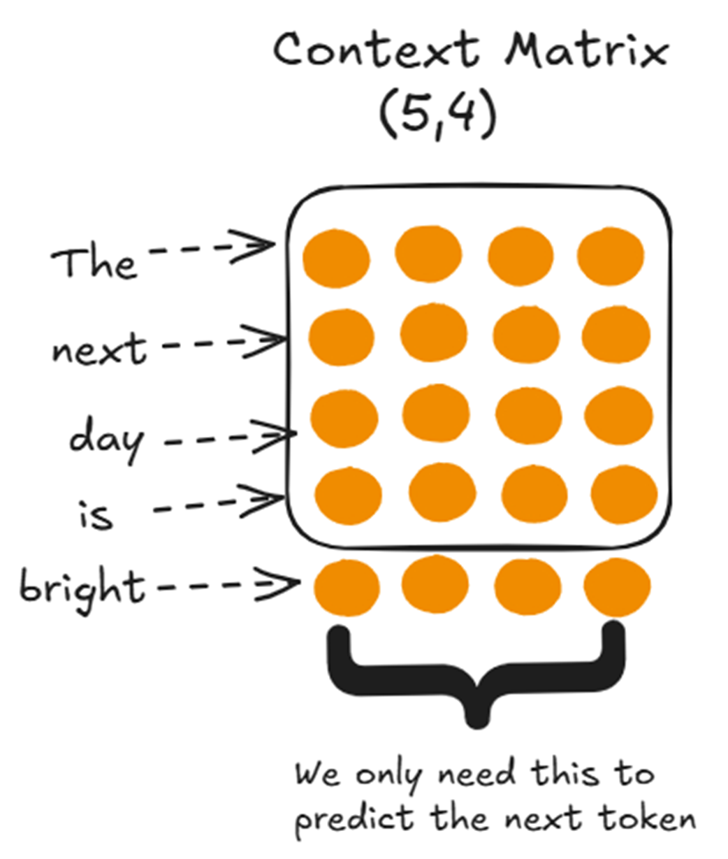
So, our immediate goal is to compute this one vector. Let’s backtrack to figure out the minimal set of computations required to produce it.

How is the Context Vector for “bright” Calculated?

From our previous exploration of the attention mechanism, we know that the context vector is the result of multiplying the attention weights by the Value matrix. Since we only need the context vector for “bright,” we only need to perform the calculation for that specific row.

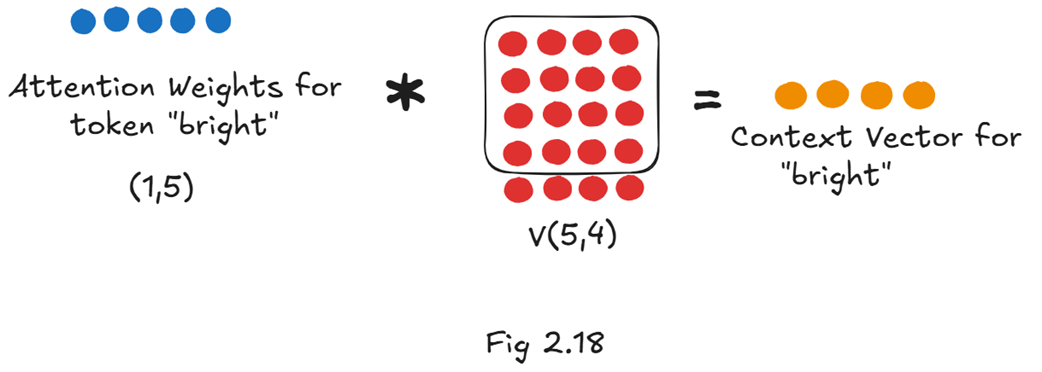
As figure 2.18 shows, to get our target vector, we need two components:

• The Attention Weights for “bright”: This is a single row vector (shape 1x5) that tells us how much “bright” should attend to every token in the sequence (including itself).
• The full Value matrix: This is a matrix of shape (5x4) that contains the “content” representation for every token in the sequence.

Let’s continue backtracking. How do we get these two components?

How are the Attention Weights for “bright” Calculated?

The attention weights are simply the softmax-normalized attention scores. So, to get the weights for “bright,” we first need the raw attention scores for “bright.” These scores are calculated by taking the dot product of the Query vector with the transpose of the full Key matrix.

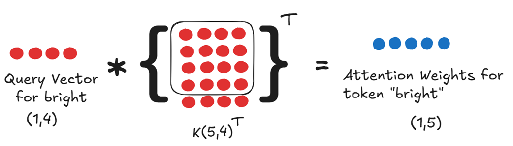
To get the attention weights, we fundamentally need:

• The Query vector for our new token.
• The full Key matrix, which contains the Key vectors for all five tokens in the sequence.

So, our list of requirements has now grown. To get the single context vector for “bright,” we need:

• The Query vector for “bright” (q_bright).
• The full Key matrix (K).
• The full Value matrix (V).

This finally brings us to the source: how are these Query, Key, and Value vectors created?

The Query, Key, and Value vectors are all created by projecting the input embeddings through the learned weight matrices Wq, Wk, and Wv. Here is where we can separate what is new from what is old.

When the new token “bright” arrives, we must compute its specific Query, Key, and Value vectors. This is done via three simple matrix multiplications using its input embedding, X_bright.

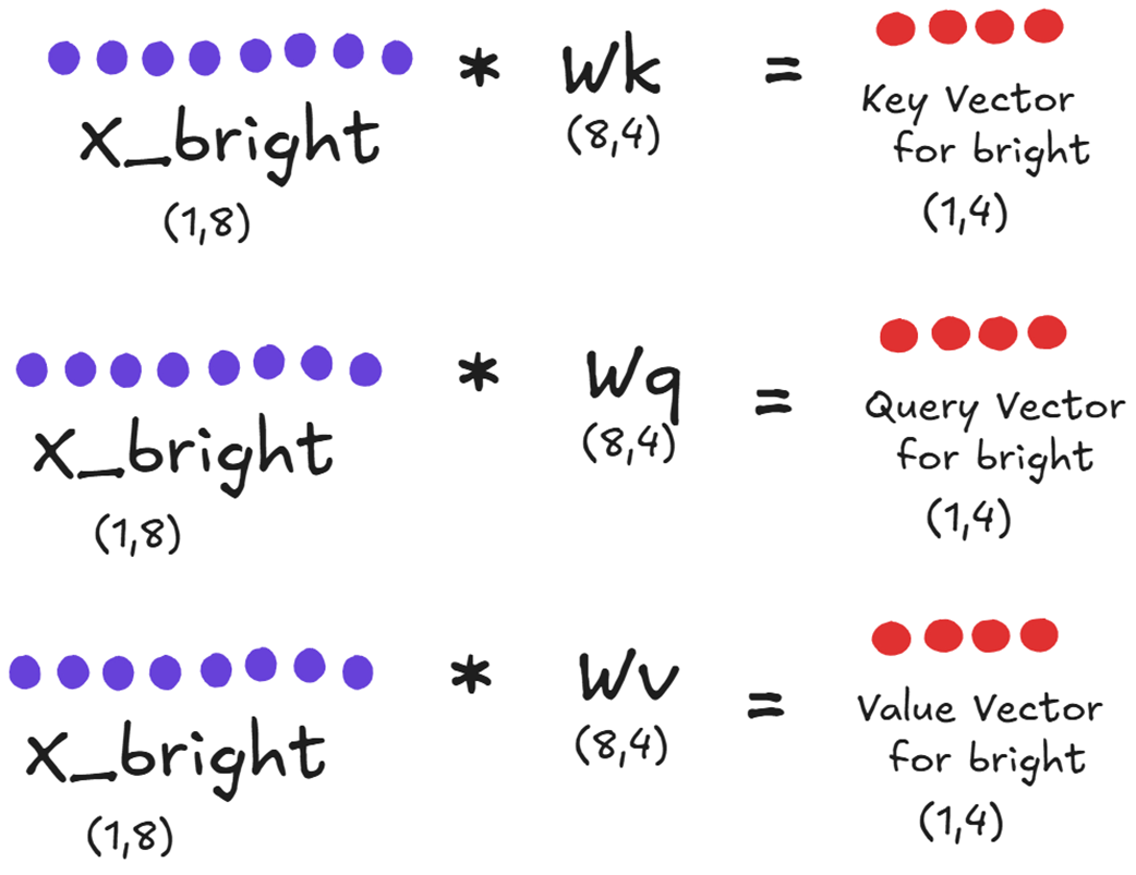
As shown in figure 2.20, these are the only new projections required:

• We compute the Query vector for “bright.”
• We compute the Key vector for “bright.”
• We compute the Value vector for “bright.”

Now we can finally answer the central question: what about the Key and Value vectors for all the previous tokens (“The”, “next”, “day”, “is”)?

In the inefficient, uncached approach we saw in section 2.3, we would have re-calculated them from scratch. But now we understand that this is wasteful. These previous Key and Value vectors have already been computed in prior inference steps. They don’t change.

This is precisely where the concept of caching comes into play. Instead of re-computing them, we can simply store the Key and Value matrices from the previous step in memory. This stored data is the Key-Value (KV) Cache. This leads us to the final, efficient workflow and answers why we only cache Keys and Values, but not Queries:

1. Compute for the New Token: When the token “bright” arrives, we perform the three essential multiplications to get its Query, Key, and Value vectors.
2. Assemble the Full Key & Value Matrices:
   • We retrieve the Key matrix for “The next day is” (a 4x4 matrix) from our KV Cache.
   • We append the new Key vector for “bright” to it, creating the full 5x4 Key matrix.
   • We do the exact same thing for the Value matrix, retrieving the old Value matrix from the Value Cache and appending the new Value vector.
3. Calculate Attention: We use the new Query vector for “bright” and the full, updated Key and Value matrices to perform the attention calculation and get the single context vector we need.
4. Update the Cache: We update our cache by storing the new, larger 5x4 Key and Value matrices, ready for the next token.

This is the essence of the Key-Value Cache. We only perform the expensive projection calculations for the single new token at each step. All historical information is preserved in the cache. We don’t need to cache the Query vectors because, as we’ve established, we only ever use the query for the current token, which must always be computed fresh. This simple but powerful technique of caching the Keys and Values is what transforms the attention calculation from a cripplingly slow quadratic operation into an efficient linear one.

2.4.2 The new inference loop with KV caching

With our understanding of what to cache, we can now define a new, highly efficient workflow for autoregressive generation. At each step, instead of re-calculating the entire history, we leverage our stored Key and Value matrices.

Let’s summarize the new process when generating a token:

1. Receive New Token: The model receives the embedding for the single, new token.
2. Compute New Projections: Perform the three essential matrix multiplications to get the Query, Key, and Value vectors for only this new token.
3. Retrieve from Cache: Load the existing Key and Value matrices for all previous tokens from the KV Cache.
4. Append to Cache: Append the new Key and Value vectors to the cached matrices to form the full, updated Key and Value matrices for the entire sequence.
5. Calculate Attention: Multiply the new Query vector with the transpose of the full, updated Key matrix to produce the raw attention scores, which are then converted into attention weights.
6. Compute Context Vector: Multiply the attention weights by the full, updated Value matrix to get the single context vector for the new token.
7. Predict Next Token: Pass this context vector through the rest of the model’s layers to predict the next token.
8. Update Cache: Save the updated Key and Value matrices back into the KV Cache for the next iteration.

This loop avoids the massive redundancy of the naive approach. The heavy lifting of matrix multiplications for past tokens is done only once and their results are simply reused. It’s important to remember that this caching happens independently at each level of the architecture: the KV cache is maintained on a per-layer and per-head basis. This means each Transformer layer in the model keeps its own distinct set of Key and Value caches for each of its attention heads, ensuring that the specialized context learned at each layer is preserved.

2.4.3 Demonstrating the speedup of KV caching

The theoretical benefit of moving from a quadratic to a linear process is clear, but the real-world impact is even more striking. We can demonstrate this with a simple test using the pre-trained GPT-2 model from Hugging Face, which allows us to enable or disable the KV cache with a simple flag (use_cache).

The following code will generate 100 new tokens from a prompt, first with the KV cache enabled, and then with it disabled, timing both processes.

Listing 2.2 Demonstrating the Speedup of KV Caching

prompt = "The next day is bright"
inputs = tokenizer(prompt, return_tensors="pt")
input_ids = inputs.input_ids
attention_mask = inputs.attention_mask
 
# Timing without KV cache
start_time_without_cache = time.time()
# Generation is performed with the KV cache explicitly disabled. 
# This forces the model to re-calculate the Key and Value matrices for the entire sequence 
# for every single token it generates, which is computationally expensive.
output_without_cache = model.generate(input_ids,
    max_new_tokens=100,
    use_cache=False,
    attention_mask=attention_mask)
end_time_without_cache = time.time()
duration_without_cache = end_time_without_cache - start_time_without_cache
print(f"Time without KV Cache: {duration_without_cache:.4f} seconds")
 
# Timing with KV cache
start_time_with_cache = time.time()
# We enable the KV cache by setting use_cache=True. 
# Now, the model only computes the projections for the newest token and reuses the cached 
# Keys and Values for all previous tokens, resulting in a dramatic speedup.
output_with_cache = model.generate(input_ids,
    max_new_tokens=100,
    use_cache=True,
    attention_mask=attention_mask)
end_time_with_cache = time.time()
duration_with_cache = end_time_with_cache - start_time_with_cache
print(f"Time with KV Cache: {duration_with_cache:.4f} seconds")
 
# Calculate and print the speedup
speedup = duration_without_cache / duration_with_cache
print(f"\nKV Cache Speedup: {speedup:.2f}x")

Running this code on a standard machine reveals the efficiency of this technique.

Time without KV Cache: 30.9818 seconds
Time with KV Cache: 6.1630 seconds
 
KV Cache Speedup: 5.03x

The results are unambiguous. By simply enabling the KV cache, we achieve a more than 5x speedup in generating 100 tokens. For very large models and much longer sequences, this speedup factor can be even more dramatic, often reaching 6x or more. This is the incredible advantage of the KV cache: it makes real-time, interactive generation feasible by eliminating the crippling cost of repeated computation.

However, this incredible speed comes at a price. Caching isn’t free. Storing these Key and Value matrices in memory introduces its own significant challenge, the “dark side” of the KV Cache.

2.5 The dark side of the KV cache: The memory cost

Now we have seen the incredible speedup the KV Cache provides. By eliminating redundant computations, it makes interactive, long-sequence generation possible. However, this efficiency comes at a steep, non-negotiable price: memory.

This isn’t just a matter of storage capacity; the inference process becomes memory-bandwidth bound. At every single generation step, the massive Key and Value matrices for all previous tokens must be read from the GPU’s main memory (HBM) into its faster compute cores. This constant data movement becomes the new performance bottleneck, which is why modern GPUs designed for AI prioritize higher-capacity HBM and greater memory bandwidth, often more so than raw computational power (FLOPS).

Caching, by its very nature, is a trade-off. We are trading memory space to save computation time. While we avoid re-calculating the Key and Value matrices, we must now store them in the GPU’s memory. For large models with long context windows, this memory footprint can become the new primary bottleneck.

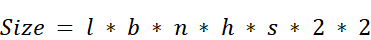
2.5.1 The KV cache formula: Deconstructing the size

We can precisely calculate the memory required for the KV cache using a straightforward formula. Figure 2.21 breaks down each component of this calculation.

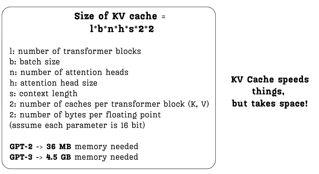
Let’s walk through the formula:

• l (layers): The total number of Transformer blocks in the model. We need a separate cache for each layer.
• u (batch size): The number of sequences we process in parallel.
• n (heads): The number of attention heads per layer.
• b (head size): The dimension of each attention head’s Key and Value vectors.
• z (sequence length): The number of tokens in the context. This is a critical factor.
• First *2: We need to cache two matrices: one for Keys and one for Values.
• Second *2: This represents the number of bytes per parameter. A standard 16-bit floating-point number (like float16 or bfloat16) takes up 2 bytes of memory.

The formula makes the trade-off explicit. Every time we want to increase the model’s context length (z), or use a larger model with more layers (l) and heads (n), the memory required for the KV cache grows proportionally.

The examples in the figure highlight the real-world impact:

• The original GPT-2 (128M) model required a relatively modest 36 MB for its KV cache.
• GPT-3, a much larger and more powerful model, requires a staggering 4.5 GB of memory for the same purpose—over 100 times more!

2.5.2 The scaling problem in practice

This exponential growth in memory consumption is a fundamental challenge in scaling Transformer models. As models grow larger and support longer context windows, the KV cache often becomes the primary limiting factor for deployment.

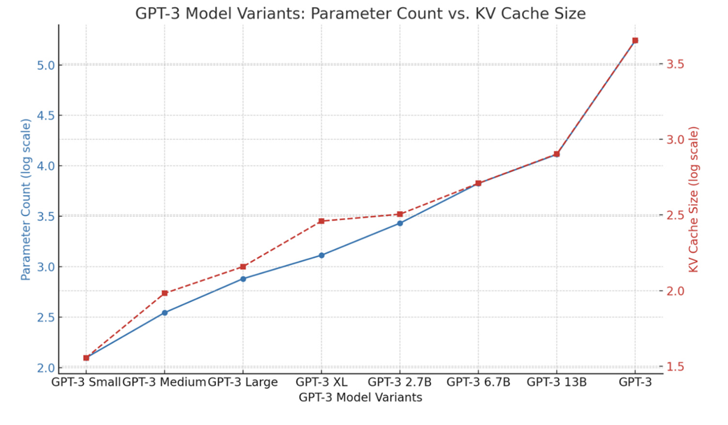
As figure 2.22 illustrates, there is a strong correlation between the size of a model and the size of its KV cache. This memory burden restricts the number of sequences we can process in a single batch and puts a hard cap on the maximum context length a model can support on a given piece of hardware.

Let’s consider two modern examples based on our notes:

For a large 30B parameter model with 48 layers, 7168 total head dimensions (n), and a context length of 1024, the KV cache for a batch size of 128 would be a massive 180 GB. This exceeds the memory capacity of even the most powerful modern GPUs.

For a model with the architectural scale of DeepSeek-V3 (61 layers, 128 heads of size 128) and a huge context length of 100,000 tokens, the KV cache for a single sequence would be approximately 400 GB.

This is the ugly side of the KV cache. It speeds things up, but it takes up an enormous amount of space. This memory pressure is the direct reason why API providers like OpenAI charge significantly more for models with larger context windows; the hardware cost to support that memory is substantial.

This bottleneck is what motivated researchers to find a better way. How can we get the speed benefits of caching without paying such a high price in memory? This question leads us to the first generation of architectural solutions: Multi-Query and Grouped-Query Attention.

2.6 The memory-first approach: Multi-Query Attention (MQA)

What is the simplest, most direct thing one could do to solve the KV Cache memory problem? Multi-Query Attention (MQA) answers this question with a radical proposal: what if all the attention heads simply share the same Key and Value matrices?

2.6.1 The core idea: Sharing a single key and value

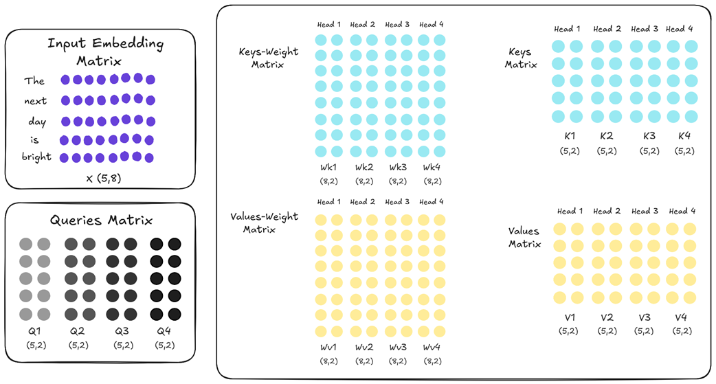
To understand MQA’s innovation, we must first recall how standard Multi-Head Attention (MHA) works. In a standard Transformer, within each layer, each attention head acts as an independent expert. This means it has its own unique, learned weight matrices for Keys (Wk) and Values (Wv), distinct from all other heads in that layer. This can be summarized as: in vanilla MHA, each head has distinct Wk and Wv.

As shown in figure 2.23, if we have four attention heads, the Key weight matrix is effectively split into four unique parts: Wk1, Wk2, Wk3, and Wk4. The same is true for the Value weight matrix. Because these weights are initialized randomly and trained independently, each head learns to project the input embeddings into a different representational space. Q1 is different from Q2, V1 is different from V2, and so on. This diversity is the source of MHA’s power; it allows the model to capture multiple perspectives simultaneously.

However, this is also the source of its memory problem. To enable fast inference, we must cache the full Key and Value matrices for every single head. Multi-Query Attention takes a direct and aggressive approach to solve this. It proposes a simple change: while each head still gets its own unique Query projection (allowing each head to “ask” a different question), all heads are forced to share one single, common set of Key and Value projections.

Look closely at the difference in figure 2.24. The Key weight matrices for all heads (Wk1 through Wk4) are now identical, and the same is true for the Value weight matrices. This means that when the input embedding is projected, the resulting K1, K2, K3, and K4 matrices are all exact copies of each other. The same applies to the Value matrices.

The implication for caching is immediate and profound. Instead of needing to store four separate Key matrices and four separate Value matrices in our cache, we only need to store one Key matrix and one Value matrix. During inference, each of the four query heads will simply attend to this single, shared set of keys and values.

This simple architectural tweak is the core idea behind Multi-Query Attention. It prioritizes memory savings above all else. In the next sections, we will explore the dramatic impact this has on the KV Cache formula and the inevitable trade-off it creates for model performance.

2.6.2 The impact on the KV cache formula

The architectural change from MHA to MQA has a dramatic and direct impact on the size of the KV Cache. Let’s revisit the formula we established in Section 2.5.1:

The key variable here is n, the number of attention heads. In MHA, because every head has its own unique Key and Value matrices, the total memory required scales linearly with the number of heads.

In Multi-Query Attention, since all heads share the same single Key and Value pair, we no longer need to store n different versions. We only need to store one. The formula becomes:

In this revised formula, the n term is effectively replaced with 1, where n is the total number of attention heads, eliminating the linear scaling with the number of heads. This reduces the size of the KV Cache by a factor of n. The impact of this reduction is staggering for large models:

GPT-3 (175B): This model has 96 attention heads (n=96). Using MQA would reduce its KV Cache size by a factor of 96, from 4.5 GB down to a mere 48 MB.

DeepSeek-V3 (671B): This model has 128 attention heads (n=128). MQA would reduce its theoretical KV Cache size by a factor of 128, from ~400 GB down to just over 3 GB.

This is an incredible reduction in memory footprint, and it directly translates to faster inference (as we will see in the code) because less data needs to be loaded from memory at each step. So, if MQA is so effective at solving the memory problem, why doesn’t every model use it?

2.6.3 The performance trade-off: Loss of expressivity

The dramatic memory savings of MQA seem almost too good to be true, and in a way, they are. This efficiency comes at a significant cost: a degradation in the model’s performance and its ability to understand complex language. To understand this trade-off, we must revisit the fundamental reason we use multi-head attention in the first place.

Let’s consider the following ambiguous sentence:

“The artist painted the portrait of a woman with a brush.”

This sentence has at least two possible interpretations:

1. Interpretation A (Instrument): The artist used a brush to paint the portrait. (painted with a brush)
2. Interpretation B (Attribute): The portrait is of a woman who is holding a brush. (woman with a brush)

A sophisticated language model needs to be able to understand and disentangle both of these potential relationships simultaneously. This is precisely what Multi-Head Attention (MHA) was designed to do.

How MHA Handles Ambiguity?

In a standard MHA block, each attention head is an independent “expert analyst” with its own set of learned weights (Wk and Wv). This independence allows them to specialize. During training, the model might learn the following:

• Head 1 could specialize in syntactic relationships. Its learned weights might cause its Key and Value vectors to focus on verb-instrument pairings. When its Query for the token “painted” looks at the Key for “brush,” it would calculate a very high attention score, effectively capturing the meaning: “The action of painting was done using a brush.”
• Head 2, on the other hand, could specialize in semantic or descriptive relationships. Its unique weights might cause its Key and Value vectors to focus on noun-attribute pairings. When its Query for “woman” looks at the Key for “brush”, it might calculate a high score, capturing the alternative meaning: “The woman in the portrait is associated with a brush.”

Because K1 is different from K2, and V1 is different from V2, the model can process both interpretations in parallel. The final context vectors contain a rich, blended understanding of all the different relationships detected by all the heads. This is the source of MHA’s expressive power.

How MQA Loses This Power?

Now, let’s consider what happens in Multi-Query Attention. MQA forces all heads to share a single, common Key and Value matrix. K1 is now identical to K2, and V1 is identical to V2.

This creates a critical problem. The single, shared Key matrix can no longer specialize. It must try to be a jack-of-all-trades, encoding a generic representation of the sentence’s information. It cannot be an expert at understanding two different kinds of relationships at the same time. For example, it struggles to precisely capture both that the brush is a tool for painting and that it is an object held by the woman.

When Head 1 (the syntax expert) and Head 2 (the semantics expert) both send out their unique queries, they are both looking at the exact same, generic set of keys. The shared Key for “brush” cannot effectively signal both “I am an instrument for painting” and “I am an object held by a woman” at the same time. One of these nuances will likely be weakened or lost entirely.

This is the fundamental drawback of MQA:

By forcing all heads to share the same Key and Value representations, MQA severely restricts their ability to specialize. The model loses a significant amount of its capacity to capture diverse and subtle relationships within the text, leading to a degradation in overall performance.

While MQA is a brilliant solution for the memory problem, it achieves this by fundamentally compromising the core strength of the multi-head design. This is why it’s often seen as a “memory-first” approach. This significant performance trade-off is what led researchers to seek a more balanced middle ground, which we will explore later with Grouped-Query Attention. But first, let’s see how we can implement this memory-saving MQA architecture in code.

2.6.4 Implementing an MQA layer from scratch

Implementing Multi-Query Attention in PyTorch is straightforward. The core logic of the attention calculation remains the same; the only change is in how the Key and Value projections are handled. Instead of creating num_heads different projections, we create only one and then repeat it for all heads.

The following code defines a MultiQueryAttention module. Pay close attention to the __init__ method, where the architectural difference is most apparent.

Listing 2.3 Implementing an MQA layer from scratch

import torch
import torch.nn as nn
 
class MultiQueryAttention(nn.Module):
    def __init__(self, d_model, num_heads, dropout=0.0):
        super().__init__()
        assert d_model % num_heads == 0, \
            "d_model must be divisible by num_heads"
 
        self.d_model = d_model
        self.num_heads = num_heads
        self.d_head = d_model / num_heads
 
        self.W_q = nn.Linear(d_model, d_model)
        # The Key and Value projections are now single, shared linear layers. 
        # They project down to the dimension of a single head (d_head) 
        # because only one projection is being created, not num_heads. 
        # This is the core architectural change that saves KV cache memory.
        self.W_k = nn.Linear(d_model, self.d_head)
        self.W_v = nn.Linear(d_model, self.d_head)
        self.W_o = nn.Linear(d_model, d_model)
 
        self.dropout = nn.Dropout(dropout)
        self.register_buffer('mask', torch.triu(
        torch.ones(1, 1, 1024, 1024), diagonal=1))
 
    def forward(self, x):
        batch_size, seq_len, _ = x.shape
 
        # The Query projection remains the same as in standard Multi-Head Attention.
        # It projects to the full model dimension, which is then split among the heads. 
        # This allows each head to "ask" a unique question.
        q = self.W_q(x).view(batch_size, seq_len, self.num_heads, 
        self.d_head).transpose(1, 2)
 
        k = self.W_k(x).view(batch_size, seq_len, 1, 
        self.d_head).transpose(1, 2)
        v = self.W_v(x).view(batch_size, seq_len, 1, 
        self.d_head).transpose(1, 2)
 
        # The single Key and Value tensors are "repeated" or broadcast to match 
        # the number of query heads. This is how all heads are made to share 
        # the same K and V information without creating expensive data copies in memory. 
        # It's the implementation of the "sharing" mechanism.
        k = k.repeat(1, self.num_heads, 1, 1)
        v = v.repeat(1, self.num_heads, 1, 1)
 
        attn_scores = (q @ k.transpose(-2, -1)) / (self.d_head ** 0.5)
 
        attn_scores = attn_scores.masked_fill(
        self.mask[:,:,:seq_len,:seq_len] == 0, float('-inf'))
 
        attn_weights = torch.softmax(attn_scores, dim=-1)
        attn_weights = self.dropout(attn_weights)
 
        context_vector = (attn_weights @ v).transpose(1, 2) \
        .contiguous().view(batch_size, seq_len, self.d_model)
 
        output = self.W_o(context_vector)
        return output

Let’s break down the key differences between this MultiQueryAttention module and a standard MultiHeadAttention module:

• Key and Value Projections: In a standard MHA, the output dimension of W_k and W_v would be d_model. Here, they project down to d_head, the size of a single head. This is because we are only creating one projection, not num_heads projections that are later split.
• Repeating K and V: The magic of MQA happens in the forward pass. After computing the single Key and Value projections, we use the .repeat() method. This doesn’t actually copy data in memory in the same way as a full matrix would; instead, it creates a “view” of the data where the same Key and Value tensors are presented to each of the num_heads Query heads. This is how “sharing” is implemented efficiently.
• Efficiency Gain: The primary gain comes from the reduced size of the Key and Value caches. In an MHA implementation, we would need to cache tensors of shape (batch_size, num_heads, seq_len, d_head) for both Keys and Values. In MQA, we only need to cache tensors of shape (batch_size, 1, seq_len, d_head), drastically reducing the memory footprint.

With this implementation, we have a functional attention layer that aggressively optimizes for memory, albeit at the cost of the performance trade-offs we’ve discussed. This sets the stage perfectly for exploring a more balanced solution.

2.7 The middle ground: Grouped-Query Attention (GQA)

This trade-off sacrificing model expressivity for memory efficiency is not ideal. It led researchers to seek a more balanced approach, a technique that could offer substantial memory savings without completely dismantling the power of the multi-head design. This solution is Grouped-Query Attention (GQA).

GQA provides a pragmatic compromise between the high expressivity of MHA and the significant memory efficiency of MQA. It lies somewhere in the middle, offering a tunable knob to balance these competing priorities.

2.7.1 The core idea: Sharing keys and values within groups

The core idea of Grouped-Query Attention is simple but effective: instead of forcing all attention heads to share the same Key and Value matrices, what if we create groups of attention heads and only share the Keys and Values within those groups?

Let’s visualize what this means. In our four-head example, instead of treating all four heads as one single unit (like in MQA), we can partition them into two groups.

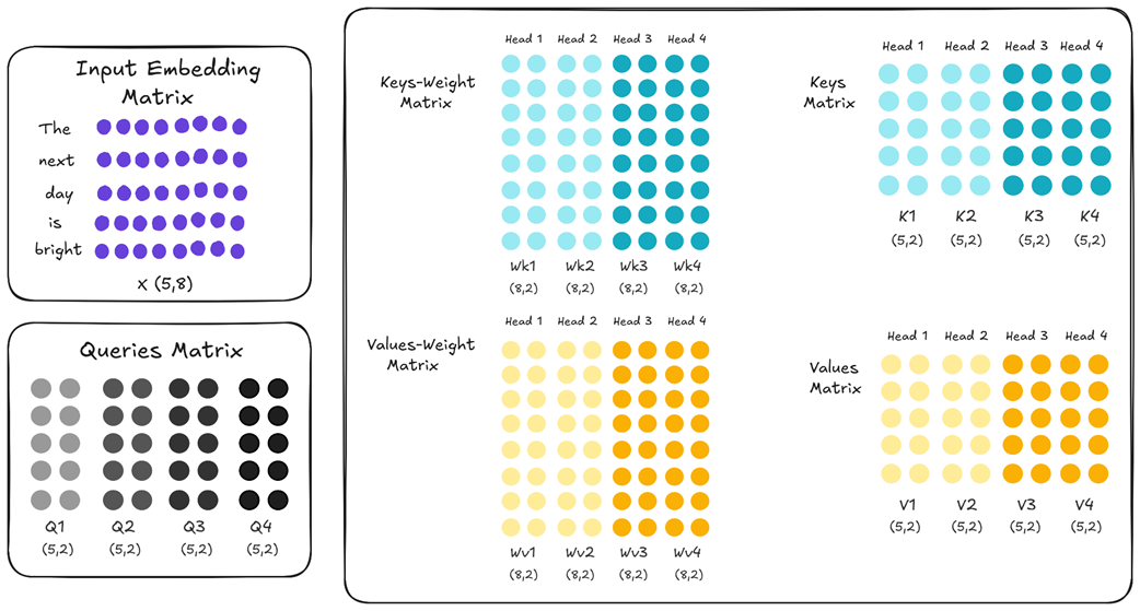
As figure 2.25 illustrates, we’ve created a hybrid model:

Within Group 1: Head 1 and Head 2 share the same Wk and Wv matrices. Their resulting K1 and K2 are identical, and V1 and V2 are identical.

Within Group 2: Similarly, Head 3 and Head 4 share their own set of Wk and Wv matrices, making K3 identical to K4, and V3 identical to V4.

Between Groups: Crucially, the K/V pair for Group 1 is different from the K/V pair for Group 2. The light blue K1/K2 matrices are distinct from the dark blue K3/K4 matrices.

This grouping strategy elegantly solves the main drawback of MQA. We are no longer forcing all heads to look at the same information. Now, Head 1 (in Group 1) and Head 3 (in Group 2) have different Key and Value matrices, allowing them to specialize and capture different perspectives, just like in standard MHA. We have reintroduced diversity into the system.

At the same time, we are still saving a significant amount of memory compared to MHA. Instead of caching four unique Key matrices, we only need to cache two: one for Group 1 and one for Group 2. GQA provides a middle ground, allowing us to find a sweet spot between model performance and memory cost.

2.7.2 The tunable knob: Balancing memory and performance

The introduction of groups in GQA provides a powerful “tunable knob” to balance the trade-off between memory efficiency and model expressivity. The number of groups, which we’ll call g, directly controls this balance.

Let’s revisit the KV Cache size formula.

• For MHA, the size scaled with n (the total number of attention heads).
• For MQA, the size scaled with 1 (a single shared K/V pair).
• For GQA, the size now scales with g (the number of unique groups).

The formula becomes:

\[Size_{GQA} = l * b * g * h * s * 2 * 2\]

This gives us a spectrum of possibilities:

• If we set the number of groups equal to the number of heads (g = n), GQA becomes identical to MHA. We have maximum performance and maximum memory usage.
• If we set the number of groups to one (g = 1), GQA becomes identical to MQA. We have maximum memory savings and the lowest performance.
• By choosing a value for g between 1 and n, we can find a practical middle ground.

For example, a model like Llama 3 8B has 32 total attention heads. Instead of the extremes of MHA (32 unique K/V pairs) or MQA (1 unique K/V pair), it uses GQA with 8 groups. This means that every 4 query heads share a single key/value head.

This reduces the KV cache size by a factor of 4 (from 32 to 8), offering a significant memory saving while retaining much more of the expressive power than MQA would. This balanced approach has made GQA a very popular choice in modern, open-source LLMs. It offers a practical way to manage the KV cache bottleneck without a crippling hit to the model’s performance.

However, it is still fundamentally a compromise. We are trading some amount of model expressivity for a reduction in memory. While GQA is a clever and effective optimization, it doesn’t solve the core tension between performance and memory; it just allows us to choose a better point on the trade-off curve.

This led the DeepSeek team to ask a different, more profound question: can we fundamentally change the nature of this trade-off? Is it possible to keep the full expressive power of having unique projections for every head (like in MHA) while also achieving significant memory reduction?

The answer to that question is yes, and the solution is Multi-Head Latent Attention. But before we start into that groundbreaking technique, let’s solidify our understanding of GQA by implementing it from scratch.

2.7.3 Implementing a GQA layer from scratch

Implementing Grouped-Query Attention is a natural extension of our MQA code. The key difference is that instead of having one shared projection for Keys and Values, we now have num_groups of them. We then ensure that the query heads within each group attend to the corresponding key/value group.

The following listing implements a GroupedQueryAttention module. The key variable to watch is num_groups, which acts as the “tunable knob.” It directly controls the number of Key and Value projections, allowing us to balance memory savings and model performance.

Listing 2.4 Implementing a GQA layer from scratch

import torch
import torch.nn as nn
 
class GroupedQueryAttention(nn.Module):
    def __init__(self, d_model, num_heads, num_groups, 
    dropout=0.0, max_seq_len: int = 0):
        super().__init__()
        assert d_model % num_heads == 0, \
            "d_model must be divisible by num_heads"
         assert num_heads % num_groups == 0, \
             "num_heads must be divisible by num_groups"
 
        self.d_model = d_model
        self.num_heads = num_heads
        self.num_groups = num_groups
        self.d_head = d_model / num_heads
 
        self.W_q = nn.Linear(d_model, d_model)
        # Instead of creating a single projection (d_head) like in MQA, 
        # we create num_groups projections. This parameter acts as a "tunable knob": 
        # if num_groups is 1, this is MQA; if num_groups equals num_heads, this becomes standard MHA.
        self.W_k = nn.Linear(d_model, self.num_groups * self.d_head)
        self.W_v = nn.Linear(d_model, self.num_groups * self.d_head)
        self.W_o = nn.Linear(d_model, d_model)
 
        self.dropout = nn.Dropout(dropout)
        # Optional causal mask pre-allocation logic...
        self._register_mask_buffer(max_seq_len)
 
    def forward(self, x):
        B, T, _ = x.shape
        
        q = self.W_q(x).view(B, T, self.num_heads, 
        self.d_head).transpose(1, 2)

        # The input is projected and reshaped into num_groups distinct Key and Value groups.
        k = self.W_k(x).view(B, T, self.num_groups, 
        self.d_head).transpose(1, 2)
        v = self.W_v(x).view(B, T, self.num_groups, 
        self.d_head).transpose(1, 2)
 
        heads_per_group = self.num_heads / self.num_groups
        
        # repeat_interleave broadcasts the K/V groups to the query heads. 
        # Each of the num_groups of Keys and Values is shared across heads_per_group queries. 
        # For example, if there are 8 query heads and 2 K/V groups, the first K/V group is shared 
        # by the first 4 query heads, and the second group is shared by the last 4 query heads.
        k = k.repeat_interleave(heads_per_group, dim=1)
        v = v.repeat_interleave(heads_per_group, dim=1)
 
        # ... rest of attention calculation ...
        attn_scores = (q @ k.transpose(-2, -1)) * (self.d_head**-0.5)
        causal_mask = self._get_causal_mask(T, x.device)
        attn_scores = attn_scores.masked_fill(causal_mask, float("-inf"))
        attn_weights = torch.softmax(attn_scores, dim=-1)
        attn_weights = self.dropout(attn_weights)
        
        context = (attn_weights @ v).transpose(1, 2).contiguous() \
        .view(B, T, self.d_model)
        
        return self.W_o(context)
 
    # Helper methods for mask management
    def _register_mask_buffer(self, max_seq_len):
        if max_seq_len > 0:
            mask = torch.triu(torch.ones(1, 1, max_seq_len, max_seq_len,
            dtype=torch.bool), diagonal=1)
            self.register_buffer("causal_mask", mask, persistent=False)
        else:
            self.causal_mask = None
 
    def _get_causal_mask(self, seq_len, device):
        if self.causal_mask is not None and \
        self.causal_mask.size(-1) >= seq_len:
            return self.causal_mask[:, :, :seq_len, :seq_len]
        return torch.triu(torch.ones(1, 1, seq_len, seq_len, 
        dtype=torch.bool, device=device), diagonal=1)

This implementation provides the “tunable knob” we discussed. By simply changing the num_groups argument, we can move seamlessly along the spectrum from MQA-like behavior (num_groups=1) to MHA-like behavior (num_groups=num_heads).

2.8 The performance vs. memory trade-off

We have now explored the first generation of solutions to the KV Cache memory crisis: Multi-Query Attention (MQA) and Grouped-Query Attention (GQA). Both techniques offer a significant reduction in the memory footprint of the KV cache, making it possible to run larger models with longer context lengths on existing hardware.

However, they both operate on the same fundamental principle: they save memory by reducing the number of unique Key and Value projections.

• MQA is the most extreme case, collapsing n unique K/V heads down to just one.
• GQA offers a more moderate compromise, collapsing n heads into g groups.

While effective, this is ultimately a trade-off. We are sacrificing the expressive power that comes from having fully independent, specialized attention heads in order to save memory. GQA allows us to choose a more palatable point on the performance-vs-memory curve, but it doesn’t change the curve itself. We are still forced to choose between maximum performance (MHA) and maximum memory efficiency (MQA), or a compromise in between (GQA).

This unresolved tension is what makes the DeepSeek architecture so innovative. The developers asked a different question: instead of reducing the number of heads, can we make the information within each head more compact? Can we compress the Key and Value matrices themselves?

This shift in thinking from reducing heads to compressing information is the conceptual leap that leads directly to Multi-Head Latent Attention, which we’ll discuss in chapter 3. It represents a fundamentally new approach to solving the KV Cache bottleneck, one that aims to preserve the full expressive power of MHA while still achieving dramatic memory savings.

2.9 Summary

• Autoregressive generation, where each new token is appended to the input, results in the re-processing of the entire sequence at every step in a naive implementation.
• This repeated computation leads to a quadratic (O(n²)) complexity problem, which makes generating long sequences of text computationally impractical.
• The Key-Value (KV) Cache optimizes inference by storing the Key and Value matrices of past tokens, avoiding redundant calculations and transforming the process into a linear-time (O(n)) operation.
• While the KV Cache dramatically accelerates computation, it introduces a severe memory bottleneck, as its size grows proportionally with sequence length, number of layers, and attention heads.
• Multi-Query Attention (MQA) drastically reduces the KV cache’s memory footprint by forcing all attention heads to share a single Key and Value projection, but this significantly degrades model performance by preventing head specialization.
• Grouped-Query Attention (GQA) provides a tunable compromise by having groups of attention heads share Key and Value projections, allowing a balance between memory savings and model expressivity.
• Architectures like MQA and GQA fundamentally operate by reducing the number of unique Key/Value pairs, establishing an inherent trade-off between memory efficiency and the expressive power of the model.