3 The DeepSeek breakthrough: Multi-Head Latent Attention (MLA)

Here is the tidied, corrected, and formatted version of the text.

This chapter covers

• Compressing the KV Cache with Multi-Head Latent Attention (MLA)
• Injecting positional awareness with Rotary Positional Encoding (RoPE)
• Fusing MLA and RoPE with a decoupled architecture

In our last chapter, we completed Stage 1 of our journey by building a solid foundation in efficient LLM inference. We began with the problem of repeated calculations, which we solved with the KV Cache. However, we then saw the dark side of the KV Cache: its massive memory cost. We explored the first-generation solutions, MQA and GQA, which help with memory usage but introduce a painful trade-off by sacrificing the expressive power of Multi-Head Attention (MHA). This left us with an unresolved tension between performance and efficiency.

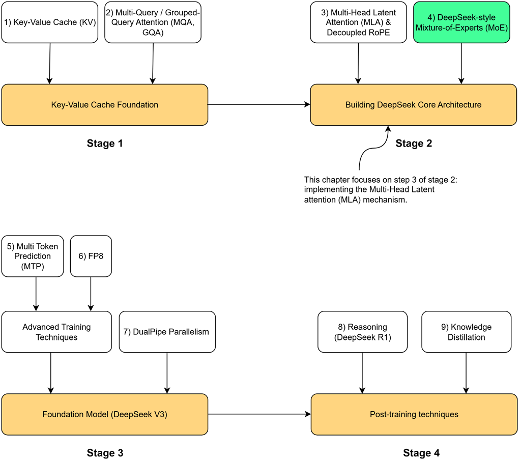
Figure 3.1 Our four-stage journey to build the DeepSeek model. Having completed the Key-Value Cache Foundation (Stage 1), we now begin Stage 2. This chapter focuses on the highlighted component, Multi-Head Latent Attention (MLA) & Decoupled RoPE, the first major innovation in the core architecture.

As highlighted in our roadmap figure 3.1, the first architectural piece we will build is Multi-Head Latent Attention (MLA). This is the core innovation DeepSeek pioneered to break the trade-off between performance and memory. First introduced in DeepSeek-V2 and carried forward to its successors, MLA proved highly effective at dramatically reducing the KV Cache footprint. However, solving the memory problem is only half the battle. To understand context, our model also needs positional awareness, which we will provide using the state-of-the-art technique, Rotary Positional Encoding (RoPE).

This brings us to the central challenge of this chapter: standard RoPE is fundamentally incompatible with MLA. To resolve this conflict, we will build a complete, production-ready attention block from the ground up, implementing the key DeepSeek innovations side-by-side.

First, we will implement Multi-Head Latent Attention (MLA). By coding the down-projection and up-projection layers, we will demonstrate how MLA dramatically reduces the KV Cache’s memory footprint while preserving the expressive power of standard Multi-Head Attention.

Second, we will tackle positional awareness by building the modern solution, Rotary Positional Encoding (RoPE). We’ll start by exploring the flaws in simpler approaches to understand why RoPE is effective, then implement its rotational mechanism from scratch.

Finally, we will combine these two concepts by implementing DeepSeek’s Decoupled RoPE architecture. This involves constructing two parallel processing paths—one for content and one for position—and then adding their outputs. This final implementation will provide a functional DeepSeek module that balances high performance with memory efficiency, forming the core of the DeepSeek model.

3.1 MLA: The best of both worlds

The state of attention mechanisms before DeepSeek presented a difficult choice. We were forced to navigate a trade-off curve: on one end, the maximum performance of Multi-Head Attention with its massive memory cost; on the other, the memory efficiency of Multi-Query Attention with its compromised expressiveness.

This led the DeepSeek team to ask a more profound question: Can we break the trade-off itself?

Is it possible to design an attention mechanism that delivers:

1. Low Cache Size: A memory footprint comparable to the highly efficient MQA or GQA.
2. High Performance: The full expressive power of MHA, where every attention head has a unique, specialized perspective.

It seems impossible. To reduce the cache size, it feels like we must reduce the amount of unique information we store. How could we possibly have different values for every head’s Key and Value without caching them all?

The answer lies in a beautiful trick, a new way of thinking about the problem. The core innovation of MLA is to shift the focus from reducing the number of heads to compressing the information within them.

The insight is this: what if we don’t have to cache the Key and Value matrices separately? What if we could first project our input into a single, combined, and much smaller matrix, a latent matrix, and cache only that?

This is the central idea of Multi-Head Latent Attention. Instead of caching two large, full-dimensional matrices ($K$ and $V$), we cache one smaller, lower-dimensional matrix ($cKV$). This single latent matrix becomes our new, highly efficient cache. Then, when we need the full Key and Value matrices for the attention calculation, we can reconstruct them on the fly from this compressed latent representation.

This is the magic of MLA:

• For Caching: We store a single, small, compressed matrix.
• For Calculation: We decompress it to get full-sized, unique Key and Value matrices for every head.

This approach promises to deliver the best of both worlds. It achieves this by cleverly factorizing the Key and Value projections into a two-step process: a compression to a smaller latent space for efficient caching, followed by a reconstruction step to the full-dimensional space for the attention calculation. To understand how it works, we must first look at the new architecture that makes this compression and decompression possible.

3.2 The MLA architecture: A visual walkthrough

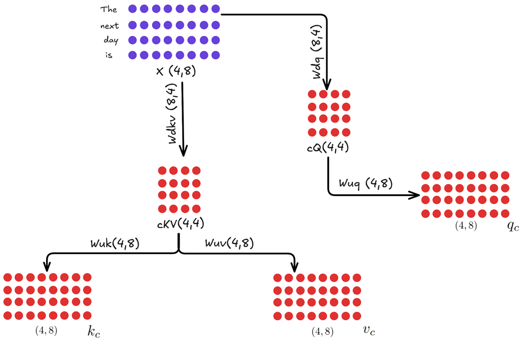
To achieve this “compress for storage, decompress for use” strategy, Multi-Head Latent Attention introduces a new set of projection layers and modifies the data flow within the attention block. Instead of projecting the input directly into Keys and Values, it first projects the input into a compressed latent space.

Let’s examine the complete workflow, as illustrated in figure 3.2.

Figure 3.2 The full architectural data flow of Multi-Head Latent Attention (MLA).

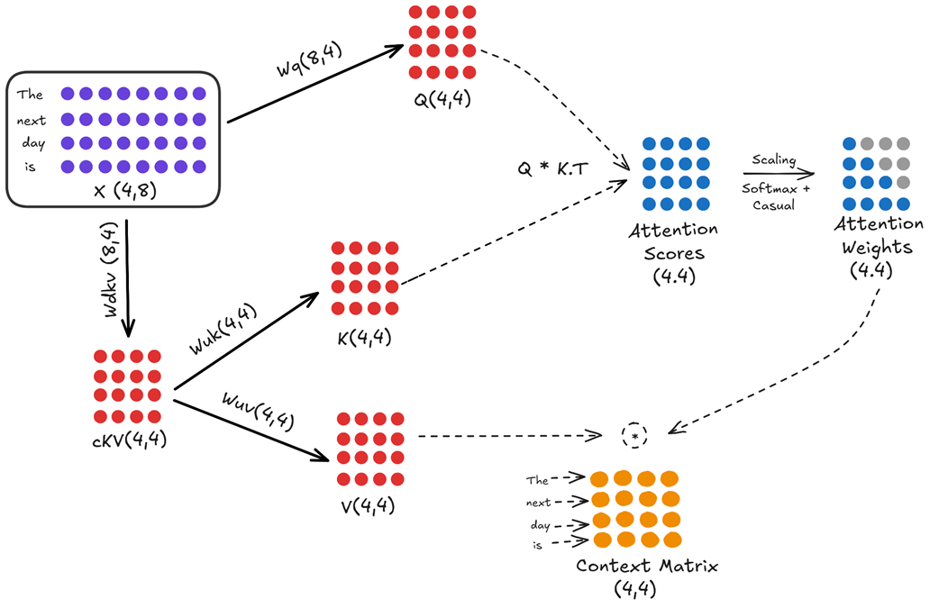
This diagram looks complex at first, but it’s a logical extension of what we already know. Let’s break it down into its two main paths: the query path and the key/value path.

3.2.1 The query path (unchanged)

The query path in this simplified version of MLA remains the same as in standard Multi-Head Attention. The goal is to create a full-sized query matrix that can ask “questions” of the entire context.

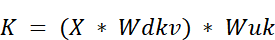
• The input embedding matrix $X$ (shape 4, 8) is multiplied by the $Wq$ weight matrix (shape 8, 4).
• This produces the final Query matrix $Q$ (shape 4, 4), ready for the attention calculation. In this example, the head dimension (d_head) is 4.

(Note: More advanced versions of MLA also compress the query, but for understanding the core KV cache innovation, we can consider the query path to be standard).

3.2.2 The key/value path (the innovation)

This is where the magic happens. Instead of two separate projections for keys and values, there is now a two-step process involving a new, intermediate latent matrix.

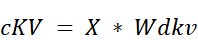
Step 1: Down-projection to the latent space

The input embedding matrix $X$ is first multiplied by a new, learnable weight matrix called the KV Down-Projector ($Wdkv$).

• $X$ (shape 4, 8) is multiplied by $Wdkv$ (shape 8, 4).
• This produces a single, smaller, compressed matrix called the Latent KV Matrix ($cKV$), with a shape of (4, 4).

Note

In our example, the latent dimension (4) happens to be the same as the number of tokens. This is purely a coincidence for the sake of simple diagrams. In practice, these dimensions are completely independent and much different. For a model like DeepSeek-V3, the model dimension is 7168 and the latent dimension is 512.

So, the KV Down-Projector ($Wdkv$) would have a shape of (7168, 512), compressing a large 7168-dimensional vector into a much smaller 512-dimensional one. The numbers in our example are kept small only to build intuition.

This $cKV$ matrix is the only thing getting cached during inference. Notice two things immediately:

• We are only caching one matrix, not two.
• The dimension of this matrix (4 in this example, but 576 in the real DeepSeek model) is much smaller than the full dimension of the Keys and Values combined.

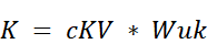
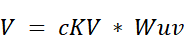
Step 2: Up-projection from the latent space

Now that we have our compressed $cKV$ matrix, we can reconstruct the full Key and Value matrices from it whenever we need them for the attention calculation. This is done with two new Up-Projection matrices:

• The $cKV$ matrix (shape 4, 4) is multiplied by the Key Up-Projector ($Wuk$ (shape 4, 4)) to produce the final Key matrix $K$ (shape 4, 4).
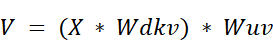
• The $cKV$ matrix (shape 4, 4) is also multiplied by the Value Up-Projector ($Wuv$ (shape 4, 4)) to produce the final Value matrix $V$ (shape 4, 4).

After this two-step process, we have our three required matrices: $Q$ (from the standard path), and $K$ and $V$ (reconstructed from the latent matrix). From this point forward, the rest of the attention calculation—computing scores, applying softmax, and calculating the context matrix—proceeds exactly as it does in standard Multi-Head Attention.

The efficiency of this method comes from a two-step process. First, we store the historical Key and Value information in a single, compressed matrix to save memory. Second, we decompress this matrix on the fly to reconstruct the full, unique Key and Value matrices for each head right when they are needed for calculation. This raises a key question: how can adding projection and reconstruction steps actually make the process more efficient? The solution is found in a specific application of matrix multiplication that we’ll refer to as the “absorption trick.”

3.3 The mathematical magic: How the latent matrix helps

We have seen the new architecture of MLA, which introduces a latent $cKV$ matrix. At first glance, this seems to add complexity. How does introducing an extra matrix and two extra projection steps ($Wdkv$ and $Wuk/Wuv$) actually lead to a more efficient system?

The answer lies in a property of matrix multiplication that the DeepSeek team exploited, a technique we’ll call the “absorption trick.” By cleverly rearranging the attention formula, we can show that the latent matrix is the only piece of historical information we need to cache, allowing us to have both a small cache and fully unique, expressive heads. To understand this, we need to write out the full sequence of calculations mathematically.

3.3.1 A Step-by-Step Derivation of Q, K, and V in MLA

Let’s formalize the steps we saw in the architectural diagram. We will use $X$ to represent our input embedding matrix.

Figure 3.3 A step-by-step mathematical derivation of the Query, Key, and Value matrices in the MLA architecture.

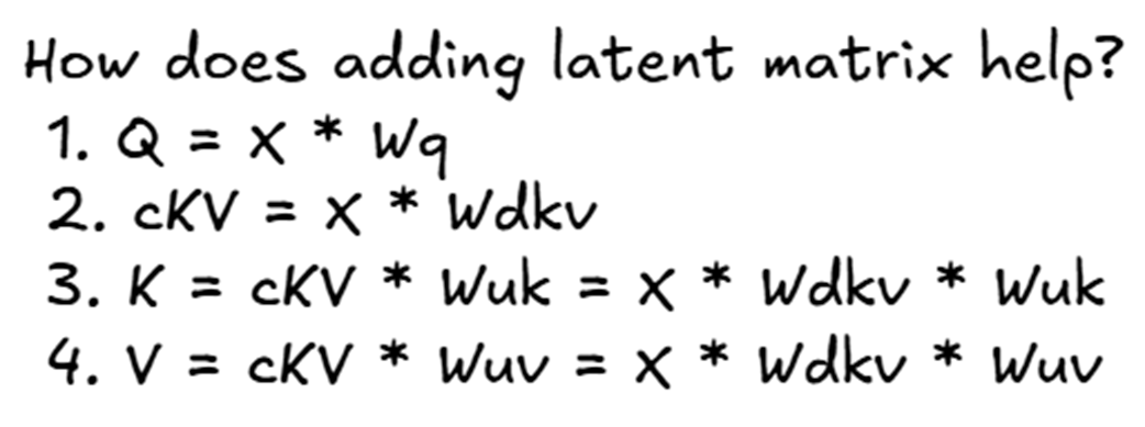
Following the steps in figure 3.3:

1. The Query Matrix ($Q$): The query calculation remains standard. It is a direct projection of the input embeddings.

2. The Latent KV Matrix ($cKV$): This is the first new step. The input embeddings are projected down into the compressed latent space. This $cKV$ matrix is what we will eventually cache.

3. The Key Matrix ($K$): The final Key matrix is no longer a direct projection of $X$. Instead, it’s an up-projection of the latent matrix $cKV$.
   • If we substitute the definition of $cKV$ from step 2, we can see the full transformation from the original input:
4. The Value Matrix ($V$): Similarly, the final Value matrix is also an up-projection of the same latent matrix $cKV$.
   • And again, substituting the definition of $cKV$:

So far, it still looks like we’ve just added extra steps. The key to understanding the efficiency gain comes when we plug these new definitions for $K$ and $V$ into the main attention score formula. This is where the magic begins.

3.3.2 The absorption trick: How attention scores are calculated

Now that we have the new mathematical definitions for our Query, Key, and Value matrices, let’s see what happens when we plug them into the core formula for attention scores:

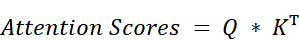
We start by substituting our new definitions for $Q$ and $K$:

Using the rule of matrix transposition $(AB)^T = B^TA^T$, we can expand the transposed term:

And applying the rule again:

This equation looks complicated, but it reveals something incredible. Notice that two of our learned weight matrices ($Wq$, $Wuk^T$) are all grouped together in the middle. Because matrix multiplication is associative, we can re-group the terms.

Figure 3.4 The mathematical rearrangement of the attention score calculation in MLA.

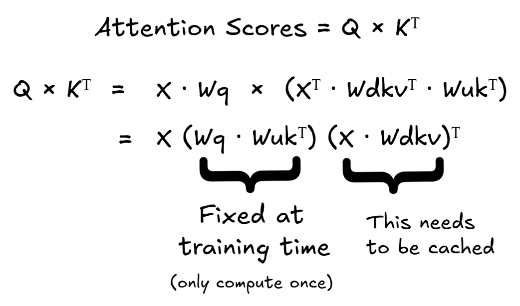
As shown in figure 3.4, we can rearrange the equation as follows:

Let’s analyze the two main components of this rearranged formula:

1. This is the product of two of our learned weight matrices. Since $Wq$ and $Wuk$ are fixed during inference (they are learned during pre-training), this entire product is also a fixed matrix. We can pre-compute it once and reuse it. It doesn’t need to be calculated at every step.
2. This term should look familiar. $X * Wdkv$ is exactly the definition of our latent KV matrix, cKV.

This is the “absorption trick.” The up-projection matrix for the Keys, $Wuk$, has been mathematically rearranged to be next to the query projection matrix, $Wq$. Because both $Wq$ and $Wuk$ are fixed, learned matrices from pre-training, their product $(Wq * Wuk^T)$ is also just a single, fixed matrix that we don’t need to re-calculate during inference.

This simplifies the process. To get our attention scores, the original formula $Q * K^T$ now effectively becomes:

This is a profound change. We started with a formula that required a full Query matrix and a full Key matrix. After this mathematical rearrangement, we see that the calculation only requires two things:

1. The original input $X$.
2. The latent matrix $cKV = X * Wdkv$.

Crucially, as we generate new tokens and our input sequence grows, the matrix $X$ representing this growing history also expands. Consequently, the latent matrix $cKV$ that summarizes this history must also expand by appending the new token’s latent vector. This proves that the $cKV$ matrix is the only piece of historical information that needs to be updated and stored to compute the attention scores. We have successfully reformulated the attention score calculation to depend only on this single, compact, cached matrix, eliminating the need to cache the full $K$ and $V$ matrices entirely.

3.3.3 The final step: Calculating the context vector

We have successfully reformulated the attention score calculation to rely on a single, cached latent matrix, $cKV$. Now, let’s see if this efficiency holds for the final step: creating the Context Vector Matrix.

The standard formula is:

We know that Attention Weights are derived from the attention scores ($Q * K^T$), which we just simplified. And we have our new definition for the Value matrix:

Let’s plug everything together.

Figure 3.5 The mathematical rearrangement for calculating the final output in MLA.

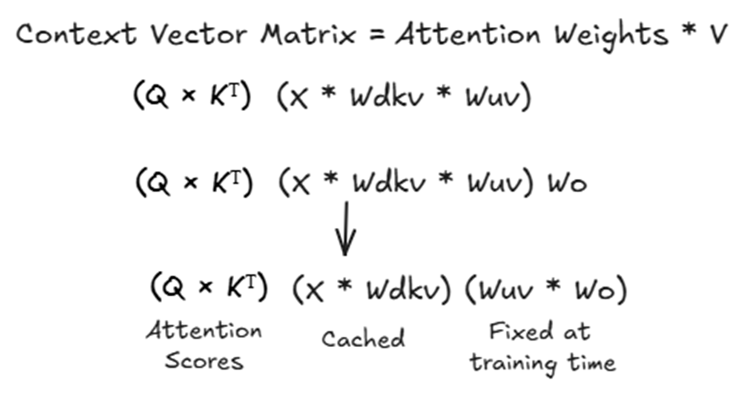
As figure 3.5 illustrates, the full calculation for the context vector, before it’s passed to the final output projection layer ($Wo$), looks like this:

Again, we can recognize the term $(X * Wdkv)$. This is our cached latent matrix.

And just like before, we can use the associative property of matrix multiplication. The $Wuv$ matrix can be “absorbed” by the final output projection layer, $Wo$. The product $(Wuv * Wo)$ is just another single, fixed matrix that is learned during pre-training.

This confirms our central thesis: we only need to cache the latent matrix.

Let’s summarize the beauty of this workflow:

1. When a new token arrives, we compute its contribution to the $cKV$ cache.
2. We use the full, updated $cKV$ cache to help compute the attention scores.
3. We also use that same, updated $cKV$ cache to help compute the final context vector.

By introducing this intermediate latent space, the DeepSeek team designed a system where a single, compact cached matrix can be efficiently used for both the key and value sides of the attention calculation. This is how they achieved the best of both worlds: a dramatically smaller memory footprint for the cache, without sacrificing the performance benefit of having unique, expressive projections for every attention head.

3.4 The new inference loop with MLA

Now that we understand the mathematical magic behind MLA, let’s put it all together and define the new, highly efficient workflow for generating a single new token. This process brilliantly leverages the cached latent matrix to avoid re-calculating the entire history.

We will trace the journey of a new token, “bright,” as it enters the system, assuming the model has already processed “The next day is” and has their latent representations stored in the $cKV$ cache.

3.4.1 What happens when a new token arrives?

The entire process is designed to be incredibly efficient, performing the absolute minimum number of computations necessary. When a new token like “bright” arrives, the model follows these steps:

Step 1: Compute the new projections

The very first step is to compute the three essential vectors for our new token. We take the input embedding for “bright,” which we’ll call $X_bright$, and perform three parallel multiplications.

Figure 3.6 Computing the Query vector for the new token.

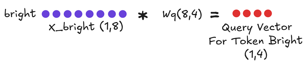
First, we compute the Query Vector for “bright”. This is a standard projection and is always calculated fresh for the current token.

Query_bright = X_bright * Wq

Next, and most importantly, we compute the token’s contribution to our new, compressed cache.

Figure 3.7 Computing the new Latent Vector cKV for “bright.”

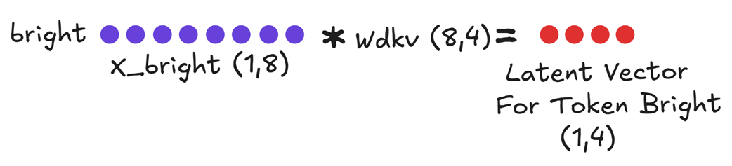
We multiply the input embedding $X_bright$ by the KV Down-Projector ($Wdkv$). This produces a single, small, compressed Latent Vector for Token Bright. This unit vector contains all the necessary Key and Value information for this token in a compressed format.

These are the only new projections we need to perform. We do not compute the full Key and Value vectors directly from the input. Instead, we will use our cache.

3.4.2 Caching the latent vector: The only thing we store

Now that we have the new Latent Vector for Token Bright, the next step is to update our cache. In the previous inference step (for the input “The next day is”), we would have already computed and stored the latent vectors for those tokens in our $cKV$ cache.

Our task now is to simply append our new latent vector to this existing cache.

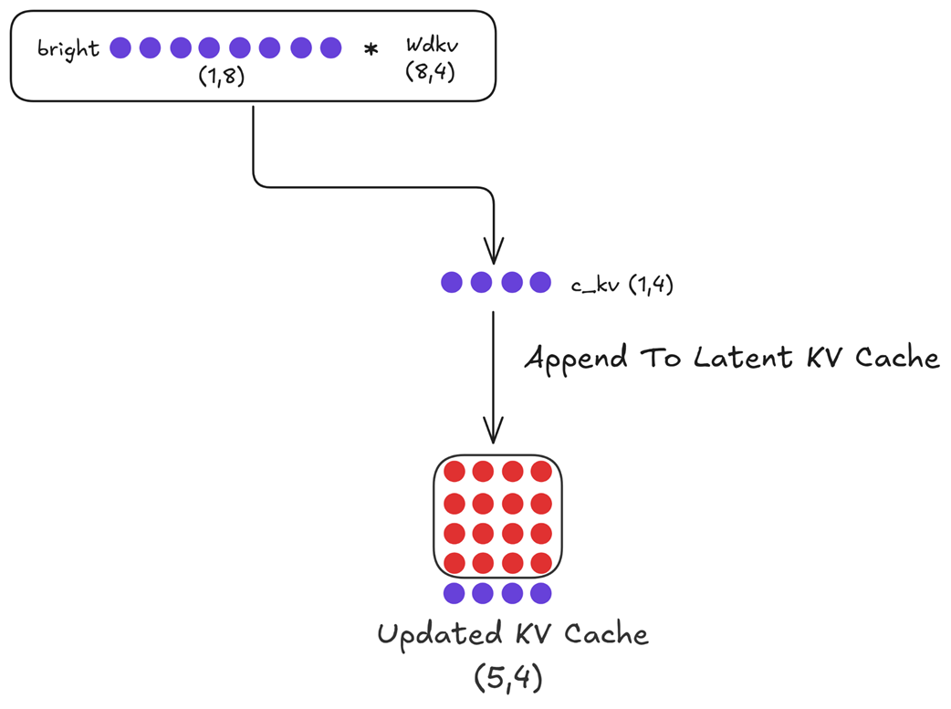
Figure 3.8 Updating the Latent KV Cache. The newly computed latent vector for “bright” is appended to the existing cache for the previous tokens.

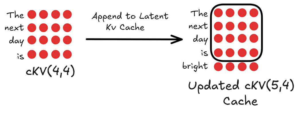
As shown in figure 3.8, our original $cKV$ cache had a shape of (4, 4), containing the compressed history. By appending the new (1, 4) latent vector, we now have an Updated latent matrix with a shape of (5, 4).

This single, compact matrix is the only piece of historical information we store in memory between steps. We do not need a separate cache for Keys and a separate cache for Values. This is the source of MLA’s memory efficiency.

3.4.3 Decompressing the cache and calculating attention

With our updated cache and the fresh Query vector for “bright” we now have everything we need to perform the attention calculation.

First, we must “decompress” our latent cache back into the full-dimensional Key and Value matrices. This is done on the fly, just for this single calculation.

Figure 3.9 Decompressing the updated latent cache into the full Key and Value matrices using the up-projection matrices.

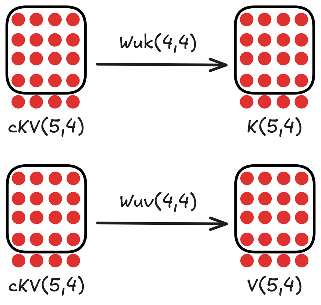
As shown in figure 3.9, we perform two parallel multiplications:

1. The Updated cKV Cache (shape 5, 4) is multiplied by the Key Up-Projector ($Wuk$) to produce the full Key Matrix $K$ (shape 5, 4).
2. The same Updated cKV Cache (shape 5, 4) is multiplied by the Value Up-Projector ($Wuv$) to produce the full Value Matrix $V$ (shape 5, 4).

Now, we have everything a standard attention mechanism needs: a fresh Query vector for our current token, and the full Key and Value matrices for the entire history, faithfully reconstructed from our compact cache.

The final steps proceed just as we’ve seen before.

Figure 3.10 The final attention calculation using the fresh Query and the decompressed Key and Value matrices.

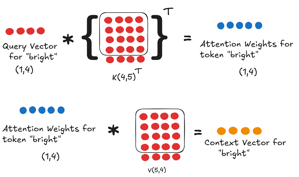
1. Calculate Attention Weights: We multiply the Query Vector for “bright” by the transpose of the full, updated Key Matrix K. The result, after scaling and softmax, is the Attention Weights for token “bright”. This is the only row we need because, as we established in chapter 2, the prediction for the next token depends only on the context vector of the last token in the sequence.
2. Compute Context Vector: We multiply these Attention Weights by the full, updated Value Matrix V to produce the single, final Context Vector for token "bright".

This single context vector is then passed through the rest of the Transformer’s layers to predict the next token. We have successfully generated our output while only ever storing the small, latent $cKV$ matrix in our cache.

3.5 Quantifying the gains

The multi-step process of MLA—compressing, caching, and decompressing—is a brilliant piece of engineering. But what does it achieve in practice? Let’s quantify the two main benefits: the reduction in cache size and the preservation of performance.

3.5.1 The new KV cache formula: A 64x reduction

In chapter 2, we established the formula for the size of a standard MHA KV cache:

The critical term was $2 * (n * h)$, representing the two separate caches (Keys and Values), each with a dimension equal to the number of heads ($n$) times the head dimension ($h$).

With MLA, this term is completely replaced. We no longer store two caches, and the dimension we store is not $n * h$, but the much smaller latent dimension, $d_latent$.

The new formula becomes:

Let’s plug in the numbers for a model at the scale of DeepSeek-V3:

• $n$ (heads) = 128
• $h$ (head dimension) = 128
• $n * h$ (total dimension) = 16,384
• $d_latent$ (latent dimension, as used in DeepSeek’s paper) ≈ 512

Let’s compare the core factors:

• MHA Cache Dimension: $2 * (n * h) = 2 * 16,384 = 32,768$
• MLA Cache Dimension: $d_latent = 512$

The reduction in the size of the cached data is: $32,768 / 512 = 64$ times.

This is an incredible achievement. By caching a single, compressed latent matrix, MLA reduces the memory footprint of the KV cache by a factor of 64. The theoretical 400 GB cache size we calculated for a DeepSeek-scale model collapses to a much more manageable ~7 GB.

3.5.2 Preserving performance: Why head diversity is maintained

More importantly, MLA achieves this massive memory reduction without the performance degradation seen in MQA and GQA. Why?

The answer lies in the up-projection matrices, $Wuk$ and $Wuv$. In the DeepSeek architecture, these up-projection matrices are themselves multi-headed. This means that there is a unique, learned $Wuk$ and $Wuv$ for every single attention head.

When we decompress the shared latent cache $cKV$, each head uses its own special up-projector. This means that:

• Head 1 reconstructs $K1$ and $V1$.
• Head 2 reconstructs a different $K2$ and $V2$.
• …and so on for all 128 heads.

At the moment of the attention calculation, every head is working with its own unique Key and Value matrices, just like in standard MHA. We have not shared any content across the heads. We have preserved the full diversity and expressive power of the multi-head design. This is how MLA achieves the best of both worlds.

3.6 Building an MLA module from scratch

Now that we have a solid grasp of the theory and the mathematical workflow of MLA, we are ready to implement it in code. We will build a PyTorch module that encapsulates the entire logic: the down-projection, the up-projection, and the final attention calculation.

For this implementation, we will focus on the core MLA mechanism itself. We will handle the caching logic outside of this module in our main inference loop, and we will address positional encodings further in this chapter.

Listing 3.1 Building MLA From Scratch

import torch
import torch.nn as nn
 
class MultiHeadLatentAttention(nn.Module):
    def __init__(self, d_model, num_heads, d_latent, dropout=0.0):
        super().__init__()
        assert d_model % num_heads == 0, \
            "d_model must be divisible by num_heads"
 
        self.d_model = d_model
        self.num_heads = num_heads
        self.d_head = d_model // num_heads # Corrected integer division
        self.d_latent = d_latent
 
        self.W_q = nn.Linear(d_model, d_model)
        self.W_dkv = nn.Linear(d_model, d_latent) # The compression layer
 
        self.W_uk = nn.Linear(d_latent, d_model) # The decompression layer for Keys
        self.W_uv = nn.Linear(d_latent, d_model) # The decompression layer for Values
 
        self.W_o = nn.Linear(d_model, d_model)
        self.dropout = nn.Dropout(dropout)
        self.register_buffer('mask', torch.triu(torch.ones(
             1, 1, 1024, 1024), diagonal=1).bool())
 
    def forward(self, x):
        batch_size, seq_len, _ = x.shape
 
        # 1. Query Path
        # The Query projection remains standard, projecting to the full model dimension before being split into heads.
        q = self.W_q(x).view(
                 batch_size, seq_len, self.num_heads, self.d_head
             ).transpose(1, 2)
 
        # 2. Key/Value Path (The MLA Innovation)
        # Down-project to the latent space (Compression)
        # This compressed c_kv is the only value that gets cached during autoregressive inference.
        c_kv = self.W_dkv(x)
 
        # Up-project from latent space to get full K and V (Decompression)
        # These values are used for the attention calculation but are not cached.
        k = self.W_uk(c_kv).view(
                 batch_size, seq_len, self.num_heads, self.d_head
             ).transpose(1, 2)
        v = self.W_uv(c_kv).view(
                 batch_size, seq_len, self.num_heads, self.d_head
             ).transpose(1, 2)
 
        # 3. Standard Attention Calculation
        attn_scores = (q @ k.transpose(-2, -1)) / \
                 (self.d_head ** 0.5)
 
        attn_scores = attn_scores.masked_fill(
                 self.mask[:, :, :seq_len, :seq_len], float('-inf'))
 
        attn_weights = torch.softmax(attn_scores, dim=-1)
        attn_weights = self.dropout(attn_weights)
 
        context_vector = (attn_weights @ v).transpose(1, 2) \
                 .contiguous().view(batch_size, seq_len, self.d_model)
 
        # 4. Final Output Projection
        output = self.W_o(context_vector)
        return output

While Multi-Head Latent Attention optimizes the Transformer’s ability to process information efficiently, the attention module is still fundamentally “time-blind.” It has no inherent sense of word order, treating sentences as a “bag of words.” For LLMs to truly understand context and generate coherent text, they need to know the position of each token. This leads us to the next crucial step on our path: positional awareness.

3.7 The problem of order

The attention mechanism, for all its power, has a fundamental limitation: it has no built-in sense of sequence order. By default, it treats a sentence as a “bag of words,” where the position of a word doesn’t matter. To the raw attention mechanism, the sentences “the dog chased the cat” and “cat the chased dog the” look identical. This is a huge problem, as the order of words is critical to the meaning of a sentence.

Let’s consider an example:

“The dog chased another dog.”

This sentence contains two instances of the word “dog.” Semantically, the token embedding for the first “dog” (the chaser) and the second “dog” (the one being chased) are identical. If we feed these token embeddings directly into the Transformer blocks without any positional information, the model has no way to distinguish between them.

As shown in figure 3.11, the input to the Transformer block for both tokens would be exactly the same. Consequently, the output context vectors produced by the attention mechanism would also be identical. The model would be blind to the fact that one dog is the subject and the other is the object. It cannot understand the true context of the sentence.

Figure 3.11 Without positional information, the Transformer processes identical tokens in different positions in the exact same way, leading to identical context vectors and a loss of crucial contextual understanding.

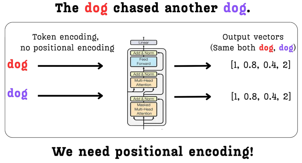
To solve this, we must find a way to tell the model where each token is located in the sequence. We need to create a distinction between the first “dog” at position 2 and the second “dog” at position 5. The mechanism for doing this is called positional encoding: we create a vector that represents a token’s position and add it to the token’s semantic embedding.

The challenge is to inject this positional information in a way that is both useful for the model and does not destroy the valuable semantic information contained in the original token embeddings. As we will see, this is a surprisingly difficult needle to thread. Let’s start by exploring the most straightforward, intuitive solution one might think of first: simply using the integer position numbers themselves.

3.8 Attempt #1: The naive approach - integer positional encodings

Now that we’ve established the critical need for positional information, let’s think from first principles. If you were tasked with designing a system to encode a token’s position, what is the simplest, most direct method you could imagine? Most likely, you would suggest using the position number itself.

3.8.1 The simple idea: Using position numbers directly

This is the core idea behind Integer Positional Encoding. We simply take the integer index of a token in the sequence and use that value to create its positional embedding.

Let’s return to our example: “The dog chased another dog.”

• The first “dog” is at position 2.
• The second “dog” is at position 5.

To create a positional embedding vector that we can add to the token embedding, we need a vector of the same dimension. If our token embeddings have a dimension of 8, we would simply create a vector where every element is the position number.

• Positional Embedding for the first “dog” (position 2): [2, 2, 2, 2, 2, 2, 2, 2]
• Positional Embedding for the second “dog” (position 5): [5, 5, 5, 5, 5, 5, 5, 5]

When we add these vectors to the identical token embeddings for “dog”, the resulting input embeddings fed into the Transformer will be different.

InputEmbedding_dog1 = TokenEmbedding_dog + [2, 2, 2, ...]
InputEmbedding_dog2 = TokenEmbedding_dog + [5, 5, 5, ...]

Problem solved, right? We are now successfully providing the model with a way to distinguish between the two dogs. The transformer will produce different context vectors for them, and it can learn the different roles they play in the sentence.

However, this simple solution introduces a new, and much more severe, problem.

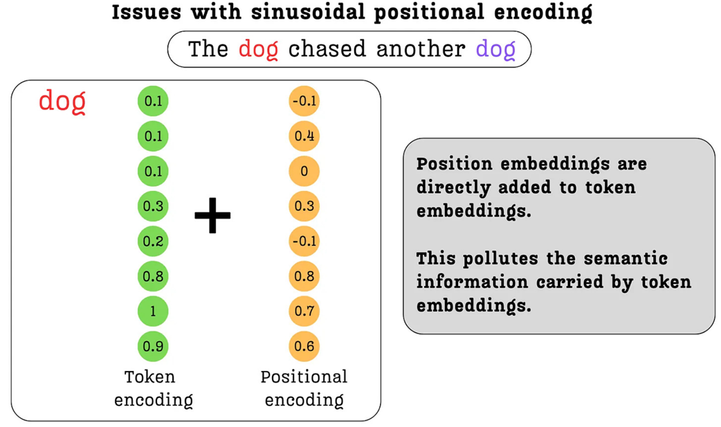
3.8.2 The major flaw: Polluting semantic embeddings with large magnitudes

The main problem with Integer Positional Encoding lies in the magnitude of the values. Token embeddings, which capture the semantic meaning of words, are typically initialized as small values clustered around zero. This is a deliberate choice in deep learning that helps with training stability. A token embedding for “dog” might look something like [0.1, 0.3, 0.2, 0.8, ...], where the values are small.

Now, consider the positional embeddings. While the values are small for the first few tokens (2, 5, etc.), what happens in a model with a large context window? A token at position 200 would have a positional embedding of [200, 200, 200, ...]. A token at position 1000 would have [1000, 1000, 1000, ...].

When we add these two vectors together, the large integer values of the positional encoding completely overwhelm the small, nuanced values of the token embedding.

Figure 3.12 The problem with Integer Positional Encoding. The large magnitude of the positional values completely dominates the small, semantic values of the token encoding, making it very difficult for the model to separate the two sources of information.

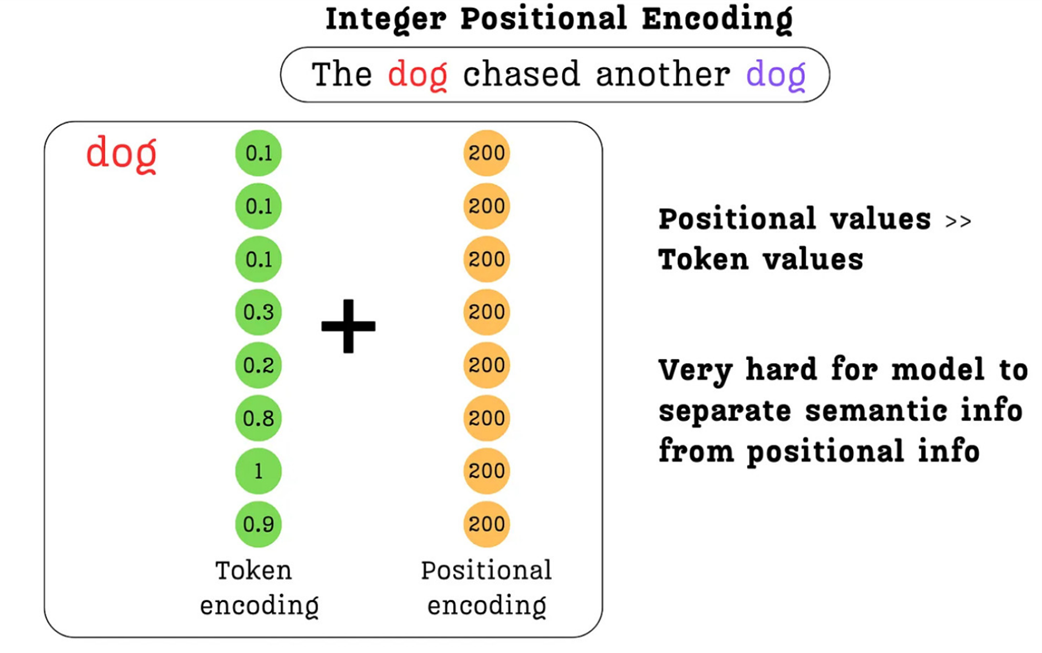
As figure 3.12 illustrates, the sum of the two vectors will be dominated by the positional information. The subtle semantic information, the very core meaning of the word “dog,” is effectively lost in the noise. We are polluting the semantics.

This defeats the purpose of having rich token embeddings in the first place. We want the model to learn from the meaning of words, but this naive approach forces the positional information to drown it out. The model would struggle to learn that the token at position 200 and the token at position 500 are related if they both happen to be the word “dog.”

Ideally, we need a method that satisfies two criteria:

1. It must provide a unique encoding for each position.
2. The values of the encoding must be constrained to a small range (e.g., between 0 and 1) so they don’t overpower the token embeddings.

This line of thinking leads directly to our second attempt: using a numerical system that is inherently constrained.

3.9 Attempt #2: A step forward - Binary positional encodings

The failure of integer positional encodings taught us a valuable lesson: the magnitude of our positional values matters. We need a system that can represent unique positions without using large, unbounded numbers that would overwhelm the semantic token embeddings.

This leads us to a natural next thought: what if we use a numerical system where the values are inherently constrained? This is the core idea behind Binary Positional Encoding.

3.9.1 Solving the magnitude problem with binary representation

Instead of using the raw integer of a position, we can represent it using its binary form. The binary system uses only two digits, 0 and 1, which perfectly solves our magnitude problem.

Let’s consider a token at position 200. If our model’s embedding dimension is 8, we can represent this position with an 8-bit binary number:

• Position 200 (Integer): 200
• Position 200 (8-bit Binary): 11001000

We can now create a positional embedding vector directly from this binary representation: [1, 1, 0, 0, 1, 0, 0, 0].

Figure 3.13 Binary Positional Encoding. The position number is converted to its binary representation, resulting in a vector of 0s and 1s that can be safely added to the token embedding without overwhelming its semantic information.

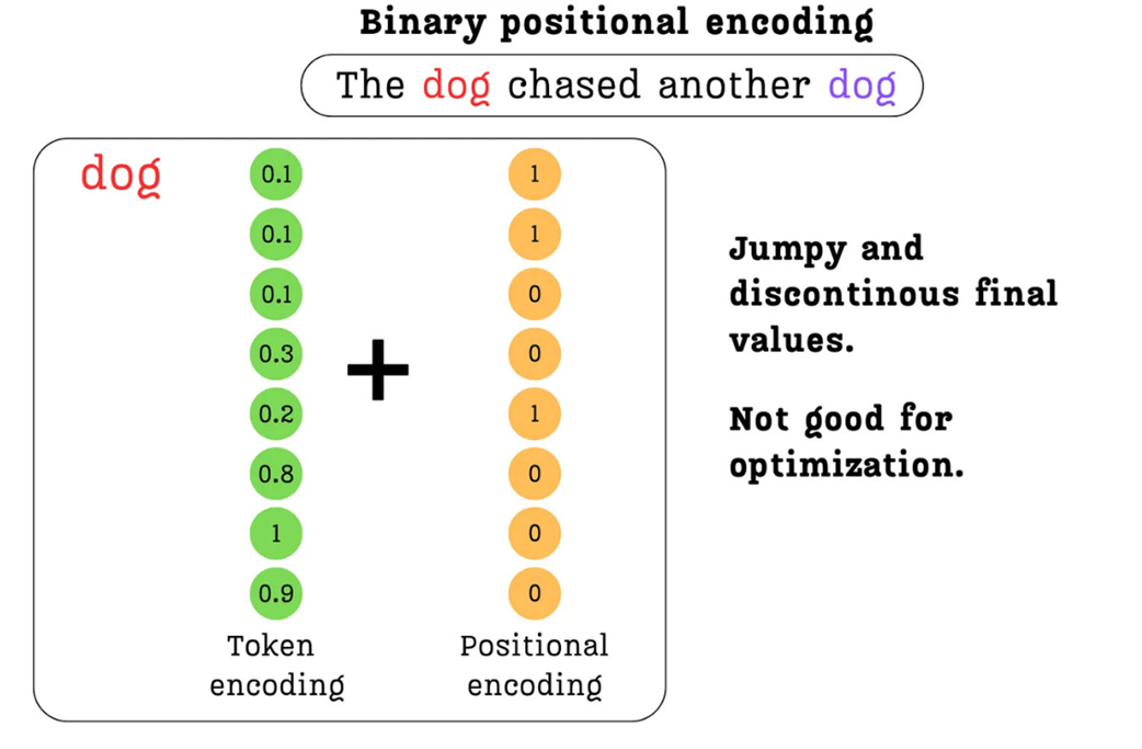
As shown in figure 3.13, this approach is a significant improvement. The positional values are now all 0s or 1s, which are on a similar order of magnitude as the small floating-point numbers in the token embedding. When we add them together, the semantic information is preserved, not polluted. We have successfully solved the primary issue with integer encodings.

This seems like a great solution. It provides a unique, fixed-length, and bounded representation for every position. However, by looking closer at the structure of these binary numbers, we can uncover a much deeper, more interesting pattern that will eventually lead us to the state-of-the-art.

3.9.2 Uncovering a deeper pattern: Oscillation frequencies

Binary positional encoding solves the magnitude problem, but it also opens the door to a new way of thinking about positions. Let’s analyze the structure of these binary numbers more closely. Within each binary representation, we can think of each digit as occupying an index, from the Least Significant Bit (LSB) on the right to the Most Significant Bit (MSB) on the left.

Figure 3.14 The oscillating frequency of bits in binary positional encodings. Lower indices (like the LSB) oscillate rapidly across positions, while higher indices (like the MSB) oscillate slowly.

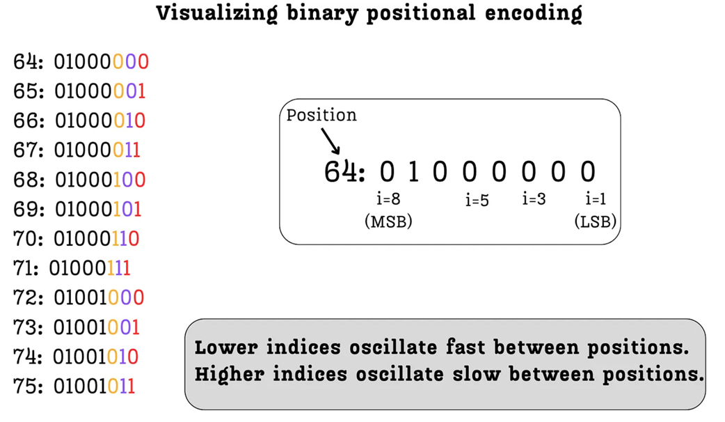
As figure 3.14 illustrates, when we look at a sequence of consecutive positions (from 64 to 75), a clear pattern emerges in how the bits at different indices change:

• Index 1 (LSB): Look at the rightmost column. The values flip at every single position: 0, 1, 0, 1, 0, 1... This bit is oscillating very rapidly.
• Index 2: The next bit flips every two positions: 0, 0, 1, 1, 0, 0... It oscillates, but at half the frequency of the LSB.
• Index 3: This bit flips every four positions: 0, 0, 0, 0, 1, 1... Its frequency is even lower.
• Index 8 (MSB): The leftmost bit doesn’t change at all in this range. It oscillates the slowest, flipping only every 128 positions.

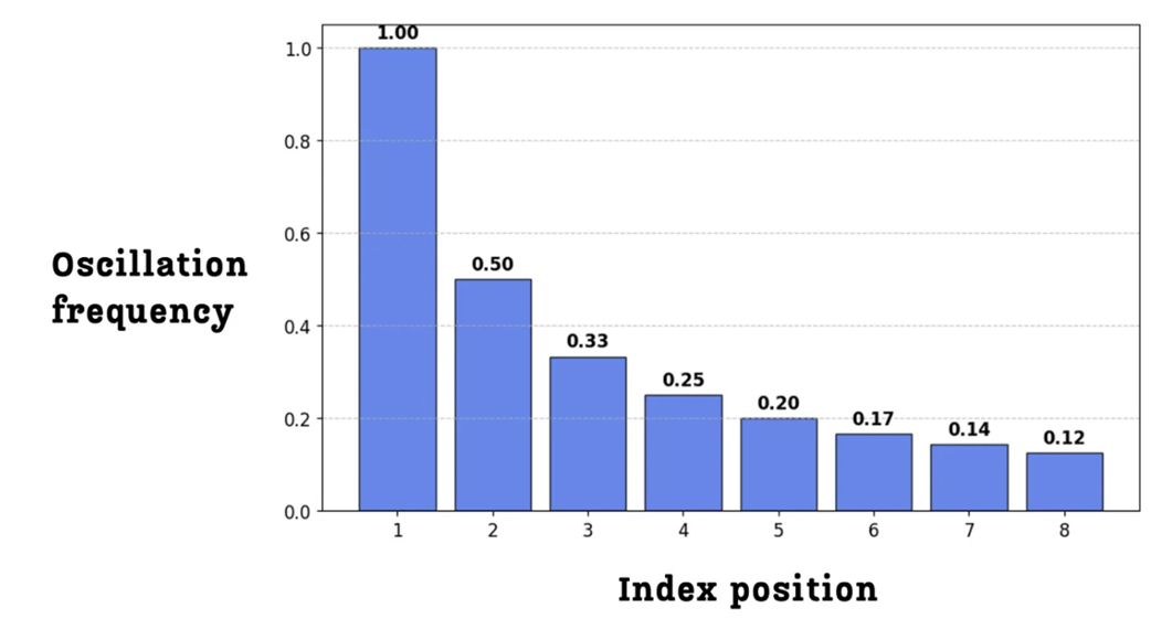
This leads us to a profound observation: lower indices oscillate fast between positions, while higher indices oscillate slow between positions. We can visualize this relationship between the index position and its oscillation frequency directly.

Figure 3.15 The oscillation frequency for each bit index in an 8-bit binary representation. The frequency is highest for the lowest index and decreases exponentially for higher indices.

This pattern can be seen even more clearly when we plot the value of each index across a longer range of positions.

Figure 3.16 The oscillation patterns of each bit index across 128 positions. Index 1 (top) oscillates very quickly, while Index 8 (bottom) oscillates very slowly.

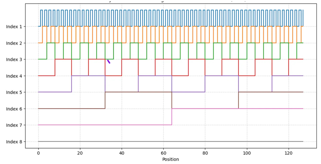
This visualization, shown in figure 3.16, is incredibly important. It reveals that binary encoding doesn’t just give each position a unique ID; it decomposes the position into a set of waves, or oscillating signals, each with a different frequency.

1. The fast-changing, low indices (like Index 1 and 2) provide fine-grained information. They are very good at distinguishing between adjacent positions (e.g., position 64 vs. 65).
2. The slow-changing, high indices (like Index 7 and 8) provide coarse-grained information. They are good at telling the model that two distant positions (e.g., 5 and 100) are far apart, as their high-index bits will be different.

This discovery that we can represent position using a combination of fast and slow oscillating signals is the key intuition that led to the development of sinusoidal and, eventually, rotary positional encodings. However, binary encoding still has one final, critical flaw.

3.9.3 The new problem: The issue with discontinuous jumps

Binary positional encoding has brought us tantalizingly close to a perfect solution. It provides a unique, bounded representation for each position and even decomposes this information into a set of meaningful, multi-frequency signals. So, what’s the problem?

The issue lies in the nature of the oscillations themselves. Look again at the plot in figure 3.16. The transition from a 0 to a 1 for any given index is instantaneous and abrupt. These are discrete jumps, creating a series of “square waves” rather than smooth curves.

These “jumpy” and discontinuous values are not good for optimization. Deep learning models, including Transformers, are trained using gradient-based optimization. This process works best when the functions involved are smooth and continuous. The sharp, step-like changes from 0 to 1 in binary encoding create a “bumpy” landscape for the optimization algorithm to navigate. It becomes difficult for the model to learn the subtle relationships between positions when the underlying positional signal is so abrupt.

Ideally, what we want is a system that keeps the brilliant multi-frequency oscillation pattern we discovered in binary encoding but makes the transitions smooth. We want a graph that has the same properties as figure 3.16, but with smooth, continuous waves instead of sharp, square steps. This immediately suggests an intuition: if we want smooth, oscillating waves, what are the most famous mathematical functions that produce them? Sine and cosine.

This exact line of reasoning is what led the authors of the original “Attention Is All You Need” paper to develop the next major innovation in positional encodings. By replacing the discrete, jumpy signals of binary encoding with the smooth, continuous waves of sinusoidal functions, they created a method that is both mathematically elegant and far more effective for training deep neural networks.

3.10 Attempt #3: The “Attention Is All You Need” breakthrough - sinusoidal positional encodings

So far we have seen that integer encodings failed due to their large, unbounded values, and binary encodings, while solving the magnitude problem, introduced undesirable discontinuities. This led us to a key insight: we need a method that can represent positions using the multi-frequency oscillating patterns of binary encoding, but with smooth, continuous values.

This is precisely the problem that the authors of the seminal “Attention Is All You Need” paper solved with the introduction of Sinusoidal Positional Encodings. This elegant technique uses the sine and cosine functions to create smooth, continuous waves that are far better suited for training deep neural networks.

3.10.1 From discrete jumps to smooth waves: Introducing sine and cosine

The core idea of sinusoidal positional encodings is to replace the jumpy 0s and 1s of binary encoding with continuous values that flow on a spectrum from -1 to 1. This is achieved using a now-famous formula that, while looking intimidating at first, is built on the same principles we’ve already discovered.

Figure 3.17 Sinusoidal Positional Encoding. The binary values are replaced with continuous values derived from sine and cosine functions, which are then added to the token embedding.

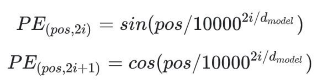
The positional encoding $PE$ for any given token depends on two variables, just as before:

• pos: The absolute position of the token in the sequence.
• i: The index of the dimension within the embedding vector.

The formula is defined in two parts:

• For even indices ($2i$), the value is calculated using a sin function.
• For odd indices ($2i + 1$), the value is calculated using a cos function.

Let’s deconstruct this. Don’t be intimidated by math. At its heart, this formula is designed to do exactly what binary encoding did: create a set of waves that oscillate at different frequencies. The term $1 / 10000^{(2i / d_model)}$ is simply the frequency of the wave.

Notice that the index $i$ is in the denominator. This means:

• For low indices (small $i$), the frequency is high, and the wave oscillates very fast.
• For high indices (large $i$), the frequency is low, and the wave oscillates very slowly.

This is the exact same property we discovered with binary encoding! Sinusoidal encodings preserve the crucial intuition of using fast-changing signals for fine-grained local information and slow-changing signals for coarse-grained global information.

Figure 3.18 Visualization of sinusoidal positional encodings for a GPT-2-sized model. The plots show the encoding values for different indices (i) across 1024 positions.

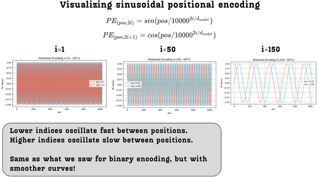
As figure 3.18 illustrates, the resulting curves are exactly what we wanted:

• They have the same multi-frequency property as binary encodings: The wave for index=1 oscillates much faster than the wave for index=150.
• They are smooth and continuous: The jumpy, discrete steps have been replaced with smooth sine and cosine waves, which are much better for the gradient-based optimization used to train LLMs.

This formula is a brilliant piece of engineering. It solves the discontinuity problem of binary encodings while preserving their most important feature. However, the use of both sine and cosine together unlocks an even deeper, more powerful property.

3.10.2 The power of rotation: Encoding relative positions

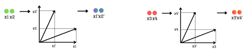
The sinusoidal formula works, but why the specific choice of pairing sin for even indices and cos for odd indices? This isn’t an arbitrary decision. This specific pairing endows the positional encodings with a remarkable property: the positional encoding for any position can be represented as a linear rotation of the encoding for any other position.

This is a crucial property. It means there is a simple, consistent mathematical relationship between the encodings of different positions. If the model can learn this simple relationship, it can generalize its understanding of positions far more effectively than if it had to memorize each position’s encoding independently.

To understand how this works, let’s visualize it. In the sinusoidal positional encoding, we can think of each pair of dimensions ($2i$ and $2i+1$) as the coordinates of a 2D vector.

• Let’s define the x-coordinate as the value at the even index ($2i$), which is $\sin(\theta)$.
• Let’s define the y-coordinate as the value at the odd index ($2i+1$), which is $\cos(\theta)$.

Here, the angle $\theta$ is determined by two factors: the token’s position in the sequence and the index of the dimension pair. The formula is:

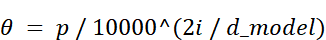
where $d$ represents the absolute position (or index) of the token in the input sequence.

Figure 3.19 A pair of sinusoidal positional encoding values can be viewed as the coordinates of a 2D vector v1 on a unit circle, defined by the angle θ.

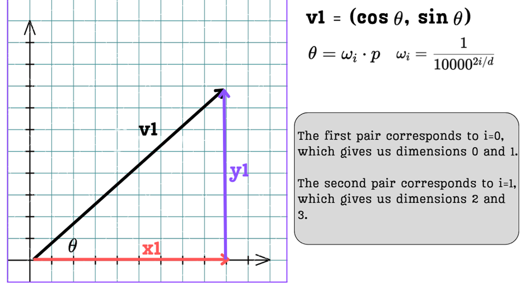
As shown in figure 3.19, for a given position $p$ and an index pair $i$, the positional encoding values form a vector $v1$ on a circle. Now, here is the puzzle: how can we find the positional encoding for a new position that is k steps away, $p + k$, using our existing encoding for position $p$?

The answer is remarkably elegant. It turns out that the positional encoding vector for position $p + k$ is simply the original vector for position $p$ rotated by a fixed angle.

Figure 3.20 The positional encoding vector v2 for a future position p + k is a simple rotation of the original vector v1 for position p.

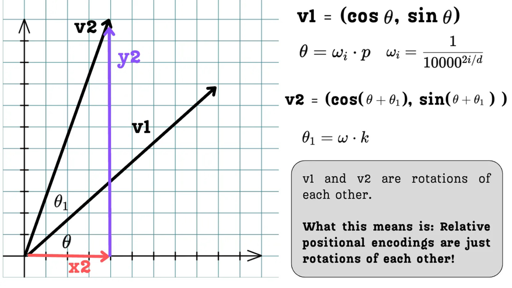
As illustrated in figure 3.20, if we want to find the positional encoding for a position that is $k$ steps away, we just need to rotate our original vector $v1$ by an angle $\theta_1 = k * \omega_i$. This is a direct consequence of the trigonometric identities $\sin(A+B)$ and $\cos(A+B)$.

This means that relative positional relationships are encoded as simple rotations. The model doesn’t need to learn complex, arbitrary patterns. It can learn that to understand the relationship between a token at position $p$ and a token at position $p+2$, it just needs to apply a consistent “two-step rotation.”

This is the genius of using the sin and cos pair.

• It provides the smooth, multi-frequency signals we need.
• It embeds a simple, linear relationship between positions, making it much easier for the Transformer to learn and generalize positional patterns.

This powerful technique, introduced in the original Transformer paper, became the gold standard for positional encodings for years. However, it still has one subtle, lingering flaw.

3.10.3 The remaining flaw: Still polluting the token embeddings

Sinusoidal positional encodings are a brilliant solution. They are continuous, they capture multi-frequency positional signals, and they encode relative positions as simple rotations. They seem to solve all of our problems. So why did the field move on to something else like RoPE?

The answer lies in how these positional encodings are integrated into the model.

If we look back at the overall architecture (Figure 3.11), we see that the positional embeddings are directly added to the token embeddings before they enter the first Transformer block.

Figure 3.21 The fundamental issue with sinusoidal positional encodings. The positional information is added directly to the token’s semantic embedding, potentially altering or “polluting” its original meaning.

As figure 3.21 highlights, even though the magnitude of the sinusoidal values is small (between -1 and 1), the very act of addition mixes the positional signal with the semantic signal. The vector that represents the meaning of the word “dog” is fundamentally altered before the model even begins to process it. This is the semantic pollution problem, or more formally representation entanglement.

It is worth noting that while this is a theoretical issue, it is not a catastrophic one. Transformers are remarkably powerful; their deep stacks of layers can learn to separate and re-interpret the mixed token and positional information. Indeed, models trained with additive sinusoidal encodings have achieved excellent performance for years. However, the core insight remained: could we find a cleaner method that avoids this entanglement from the start?

Ideally, we want the semantic information from the token embeddings to be preserved as cleanly as possible. This led researchers to ask a critical question: must we inject positional information at the very beginning?

The attention mechanism is the part of the model where the relationships between tokens and thus their relative positions truly matter. The influence of one token on another is quantified by the interaction between their Query and Key vectors.

Figure 3.22 The attention score calculation. The influence of one token on another is quantified by the dot product of their respective Query and Key vectors. This core interaction is where relative position truly matters.

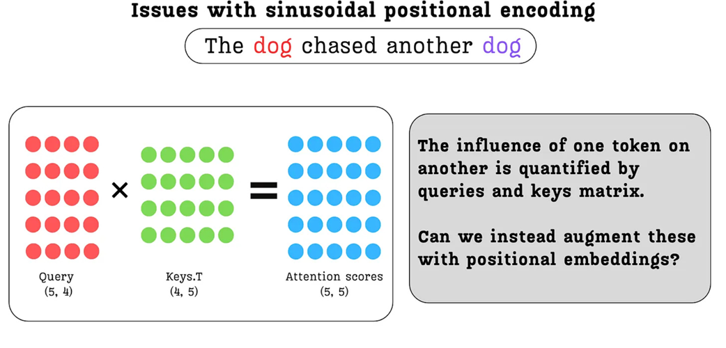
This insight, prompted by the diagram in figure 3.22, is the final step in our journey. The diagram reminds us that the entire measure of relevance between tokens boils down to the interaction between their Query and Key vectors. This begs a critical question: if this is where positional relationships are quantified, why are we modifying the token embeddings at the very beginning?

This leads to a new, cleaner approach:

1. Don’t touch the initial token embeddings. Let them carry pure semantic information into the Transformer blocks.
2. Inject positional information later, directly into the Query and Key vectors right before the attention scores are calculated.

But how should we inject this information? If we simply add a positional vector to the Query and Key vectors, we might still change their magnitude and alter their learned representations. This leads to the final, elegant idea.

Figure 3.23 The core ideas of RoPE. We can avoid polluting the original vectors by rotating them instead of adding to them, and we can apply this rotation directly to the Query and Key vectors where positional information is most relevant.

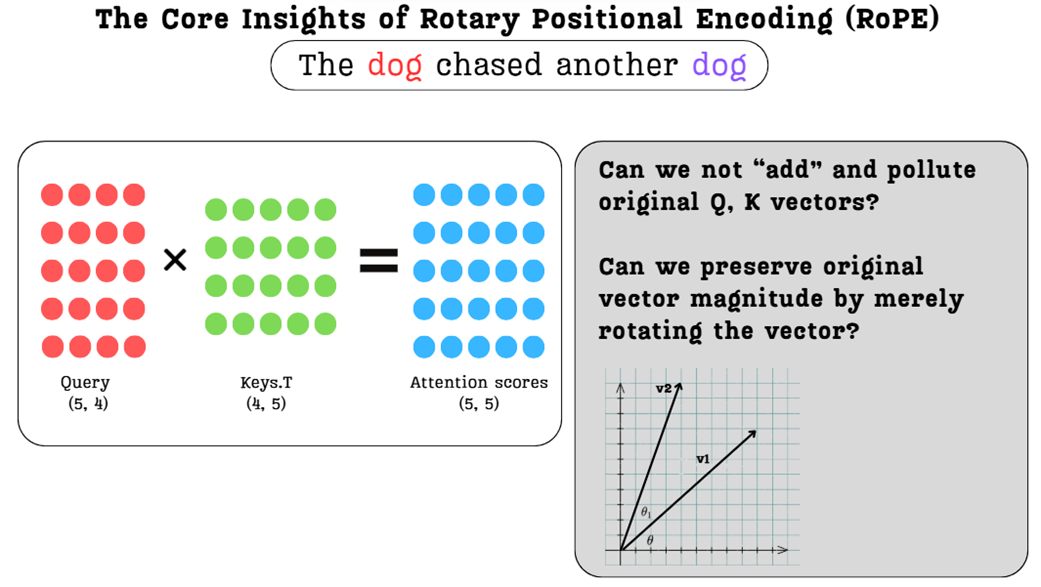
As figure 3.23 suggests, what if we combine the best ideas we’ve discovered?

• What if we inject the positional information directly into the Query and Key vectors?
• And what if, instead of adding a vector, we simply rotate them, preserving their original magnitude and learned semantic direction?

These two ideas together form the foundation of Rotary Positional Encoding (RoPE), the state-of-the-art technique that we will now explore in detail.

3.11 The state-of-the-art: Rotary Positional Encoding (RoPE)

We have seen the flaws in naive approaches and the brilliance of sinusoidal encodings, which introduced the powerful concept of encoding relative positions as rotations. However, sinusoidal encodings still suffer from one lingering issue: they pollute the semantic token embeddings by being added to them directly at the start of the Transformer block.

This is where Rotary Positional Encoding (RoPE) enters the picture. RoPE takes the best ideas from sinusoidal encodings and refines them into a more elegant and effective solution. It is built on two simple but profound insights that address the final remaining problem.

3.11.1 The core insights: Injecting position into attention and preserving magnitude

The development of RoPE started from answering two fundamental questions:

Question 1: Where is the best place to add positional information?

The attention mechanism is the part of the model where the relationships between tokens, and thus their relative positions, truly matter. The influence of one token on another is quantified by the interaction between their Query and Key vectors. Instead of modifying the token embeddings at the very beginning, why not inject the positional information directly into the Query and Key vectors, right where it’s needed most? This would allow the pure, semantic information from the token embeddings to flow into the Transformer block untouched.

Question 2: How can we add this information without corrupting the vectors?

When we add a positional vector to a token embedding, we change its magnitude and direction in vector space. This “pollutes” the original semantic representation. Is there a way to modify a vector to encode new information while preserving its original length and, to some extent, its core direction? The answer is rotation. If we simply rotate a vector, we change its coordinates, but its magnitude remains unchanged.

These two ideas together form the foundation of Rotary Positional Encoding:

Instead of adding a positional vector to the initial token embeddings, RoPE rotates the Query and Key vectors directly within the attention mechanism. The angle of rotation is determined by the token’s position.

This approach is brilliant because it solves both problems at once. We avoid semantic pollution by modifying the Q and K vectors later in the process, and we preserve the vectors’ learned magnitudes by using rotation instead of addition. In high-dimensional vector spaces, the direction of a vector captures its core semantic meaning. By only rotating the vectors, we change their orientation to encode positional information without altering their length (magnitude) or fundamentally distorting their learned semantic direction. This ensures the model’s understanding of a token’s meaning remains intact while being augmented with positional context.

Now, let’s see how this is implemented in practice.

3.11.2 The mechanism: Rotating query and key vectors

Now that we have the core idea rotating Query and Key vectors we need to understand the mechanics of how this is actually done. If you understand this mechanism, you’ll never forget RoPE, because it’s a very visual and intuitive concept. The process can be broken down into a few simple steps. For this demonstration, we will focus on a single Query vector (the exact same process applies to the Key vectors as well).

Step 1: Grouping the vector into pairs

The rotation operation is a 2D concept. However, our Query and Key vectors are high-dimensional (e.g., a 4-dimensional vector in our simplified example). How can we rotate a 4D vector?

RoPE’s clever solution is to not treat it as a single 4D vector at all. Instead, it groups the dimensions into pairs. For this example, let’s assume the dimension of a single attention head (head_d) is 4. We will be working with the individual Query or Key vector for a single token within this head.

Figure 3.24 The dimensions of a Query or Key vector are paired up for rotation.

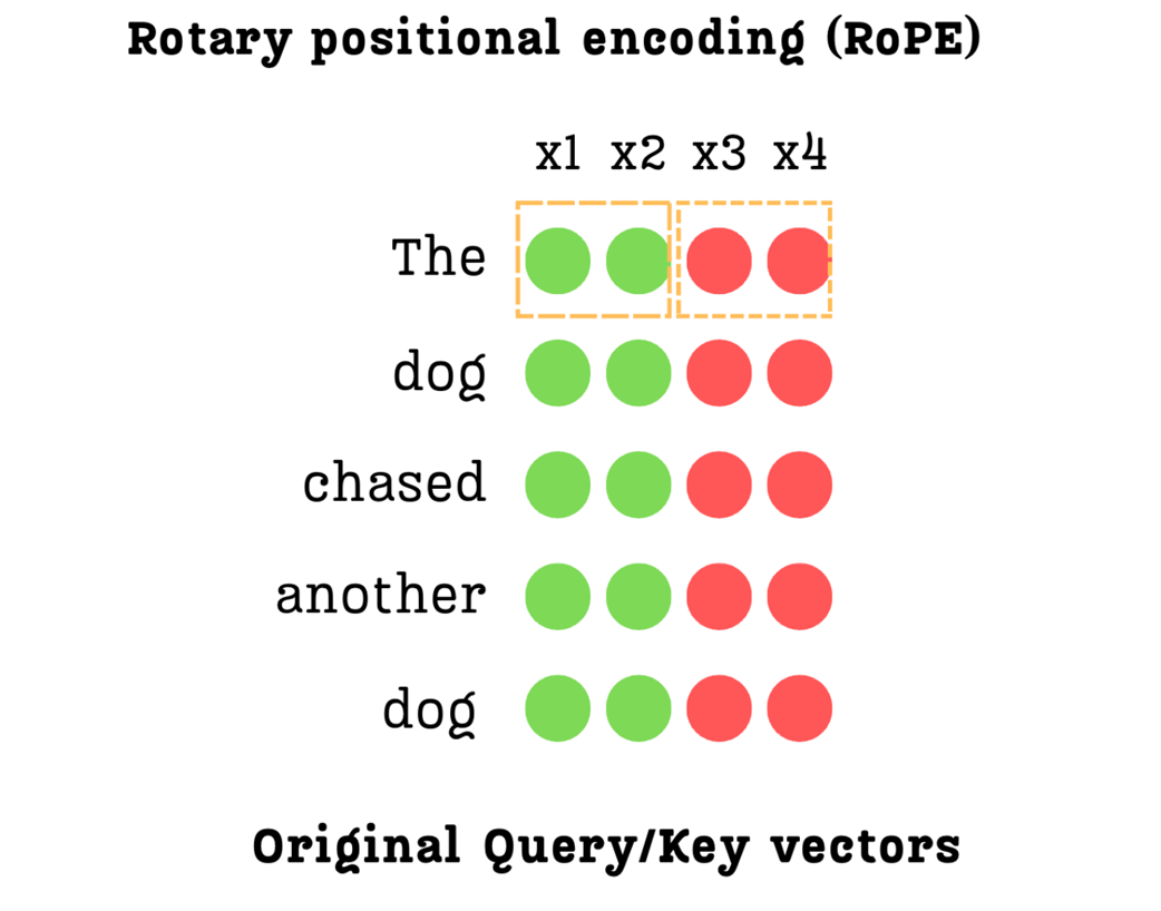
As shown in figure 3.24, for a 4-dimensional vector [x1, x2, x3, x4], we create two independent 2D groups:

• Group 1: Consists of the first two dimensions, (x1, x2).
• Group 2: Consists of the next two dimensions, (x3, x4).

Each of these pairs will now be treated as a 2D vector that we can rotate on a plane. This process is repeated for the entire length of the vector. If the vector were 128-dimensional, we would have 64 pairs to rotate.

Step 2: Rotating each pair by a position-dependent angle

With our dimensions grouped into 2D pairs, we can now apply the rotation. Each pair is rotated by an angle, $\theta$, which encodes the token’s position.

Figure 3.25 Each pair of dimensions is treated as a 2D vector and rotated by a position-dependent angle θ.

As illustrated in figure 3.25, the process for each group is identical:

• The pair (x1, x2) is treated as a 2D vector. It is then rotated by an angle $\theta$ to produce a new vector with coordinates (x1', x2').
• Simultaneously, the pair (x3, x4) is treated as another 2D vector. It is rotated by a different angle to produce (x3', x4').

This rotation is the core of RoPE. It injects the positional information into the vector. But what determines the angle of rotation?

The angle $\theta$ is calculated using the exact same logic we discovered in sinusoidal encodings. It depends on two things: the token’s absolute position ($p$) and the index of the pair ($j$).

Figure 3.26 The formula for the rotation angle θ.

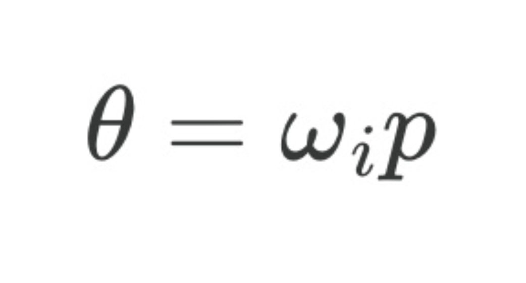
The formula is $\theta = p * \omega_i$, where $\omega_i = 1 / 10000^{(2j / h)}$.

Let’s break this down:

• $p$: The absolute position of the token (e.g., 0, 1, 2, …). A token further down the sequence will have a larger $p$, and thus a larger base rotation.
• $j$: The index of the pair we are rotating. For the first pair (x1, x2), j=0. For the second pair (x3, x4), j=1, and so on.
• $h$: The total dimension of the vector (in our case, 4).

This formula brilliantly re-implements the multi-frequency oscillation pattern.

• The first pair ($j=0$) will be rotated with a high frequency, changing significantly with each new position $p$.
• The second pair ($j=1$) will be rotated with a lower frequency, changing more slowly across positions.

This is how RoPE preserves the crucial property of using fast oscillations to capture fine-grained local relationships and slow oscillations to capture coarse-grained, long-range dependencies.

Step 3: Assembling the final position-encoded vector

After rotating each pair of dimensions independently, we reassemble them to form the final, position-encoded Query or Key vector.

Figure 3.27 The final step of the RoPE mechanism. The rotated 2D pairs are reassembled to create the final position-encoded Query or Key vector.

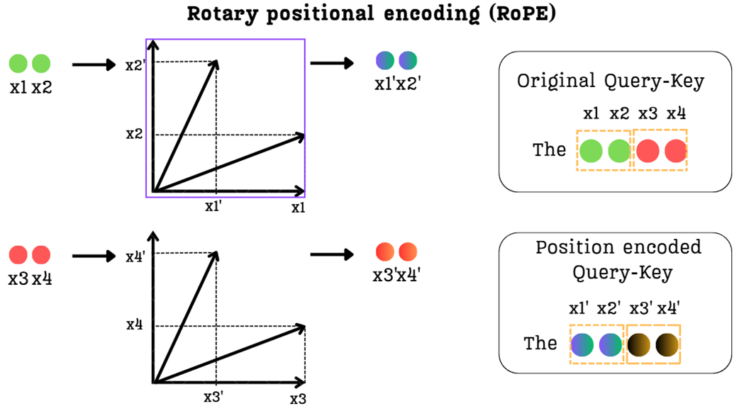
As shown in figure 3.27, the original vector [x1, x2, x3, x4] is transformed into the new vector [x1', x2', x3', x4'].

This new vector is a masterpiece of information engineering. It has successfully encoded the token’s positional information directly into its structure, and it has done so while achieving two critical goals that previous methods could not.

Benefit 1: Magnitude is preserved

The most important property of a 2D rotation is that it does not change the length (the magnitude) of the vector.

• The magnitude of the vector (x1, x2) is the same as the rotated vector (x1', x2').
• The magnitude of the vector (x3, x4) is the same as the rotated vector (x3', x4').

Because we are only rotating parts of the original vector, the overall magnitude of the final vector is preserved. This is a huge advantage. It means we can inject rich positional information without distorting the learned semantic representations of our Query and Key vectors. We have solved the “semantic pollution” problem.

Benefit 2: Relative positions are encoded

Just like with sinusoidal encodings, the use of rotation means that the relationship between two tokens at different positions can be expressed as a simple, linear transformation. The attention score between a Query at position $m$ and a Key at position $n$ will depend on their relative distance ($m-n$), which is encoded in the difference of their rotation angles. This allows the model to learn relative positional relationships in a much more natural and generalizable way.

This is the complete geometric intuition of Rotary Positional Encoding. It is an incredibly elegant solution that combines the best ideas we’ve seen so far:

• It injects positional information directly into the Query and Key vectors, avoiding the need to modify the initial token embeddings.
• It uses rotation to preserve the magnitude of the original vectors.
• It re-uses the brilliant multi-frequency formula from sinusoidal encodings to capture both fine-grained and coarse-grained positional relationships.

This powerful and efficient mechanism has become the standard for most modern, high-performance LLMs. However, as we will see, integrating this elegant solution with the equally innovative MLA architecture from DeepSeek presents one final, fascinating challenge.

3.12 The new challenge: Why standard RoPE and MLA don’t mix

We have now mastered two of the most important innovations in modern Transformer architecture:

1. Multi-Head Latent Attention (MLA): A brilliant solution for the KV Cache memory bottleneck that works by caching a single, compressed latent representation of the Keys and Values.
2. Rotary Positional Encoding (RoPE): An elegant solution for encoding positional information by rotating the Query and Key vectors before the attention calculation.

Individually, each of these techniques is a well-crafted engineering solution. The natural next step would be to combine them to create a truly state-of-the-art attention block. However, when we try to do this, we run into a fundamental incompatibility.

Let’s think about the logical flow. The standard RoPE implementation requires us to rotate the Key vectors based on their absolute position before we compute attention. But the core idea of MLA is to compute a position-agnostic latent representation of the Keys that we can store in a cache.

Herein lies the conflict:

• RoPE says: “I need to modify every Key vector differently based on its unique position in the sequence.”
• MLA’s cache says: “I need to store a simple, compressed representation that doesn’t depend on position, so I can decompress it efficiently.”

If we apply RoPE to the Key vectors before we try to compress them with MLA’s down-projector, the compression will fail. The down-projector would have to learn to “un-rotate” every vector’s unique positional information before it could compress the underlying content, which is an impossibly complex task. The beautiful simplicity of the latent cache is broken.

Conversely, if we apply RoPE after decompressing the cache, it’s too late. The attention calculation is the very next step, and we would have to re-compute the rotation for every key in the entire history at every single step, which would completely negate the speed benefits of caching.

This incompatibility between the position-dependent nature of RoPE and the position-agnostic requirement of the MLA cache is the final puzzle we must solve. The DeepSeek team’s solution to this problem is a clever and elegant modification to the RoPE mechanism itself, which we will build from scratch further in this chapter.

3.13 The incompatibility problem: Why standard MLA and RoPE don’t work together

To see exactly why standard MLA and RoPE don’t work together, we must look at the mathematics of the “absorption trick” that makes MLA so efficient.

As we established, the efficiency of MLA comes from a clever mathematical rearrangement of the attention score formula. The original formula $Q * K^T$ was transformed into:

This trick works because the two weight matrices, $Wq$ and $Wuk$, are adjacent to each other. Their product, $(Wq * Wuk^T)$, can be pre-computed as a single, fixed matrix. This allows the model to avoid caching the full Key matrix and instead only cache the much smaller latent matrix, $cKV = X * Wdkv$. This absorption is only possible because the weight matrices are position-agnostic; their values do not change based on a token’s position.

Now, let’s recall how RoPE works. It injects positional information by applying a rotation function, RoPE(), directly to the Query and Key vectors after they have been projected.

Q_rotated = RoPE(Q, position)
K_rotated = RoPE(K, position)

Crucially, the RoPE() function is position-dependent. The rotation applied to the vector for a token at position 5 is different from the rotation applied to a token at position 10.

Herein lies the problem. If we try to combine these two techniques naively, the RoPE() function ends up sitting directly between the two matrices we need to absorb. The attention score calculation would look something like this:

The position-dependent RoPE() function acts as a barrier, preventing $Wq$ and $Wuk$ from being multiplied together. The absorption trick is broken.

This has bad consequences for inference efficiency. Without the absorption trick, we would be forced to re-compute the full, rotated Key matrix for every token in the entire history at every single generation step. This would completely negate the speed benefits of caching and defeat the entire purpose of MLA.

This incompatibility between the position-dependent nature of RoPE and the position-agnostic requirement of the MLA cache is the final puzzle we must solve. The DeepSeek team’s solution to this problem is a clever and elegant modification to the architecture itself, which we will now build from scratch.

3.14 The DeepSeek solution: Decoupled rotary position embedding

To solve the incompatibility between MLA and RoPE, the DeepSeek team devised an elegant solution: if the positional information is breaking our absorption trick, let’s simply take it out of the main path. This is the core idea behind Decoupled Rotary Position Embedding.

The insight is to split the attention calculation into two parallel streams:

1. A Content Path: This path is responsible for understanding the semantic meaning of the tokens (“what”). It will use a pure, standard MLA mechanism without any positional information, allowing the absorption trick to work perfectly.
2. A Position Path: This path is responsible for understanding the relative order of the tokens (“where”). It will use a new, specialized set of projections where RoPE can be applied freely.

The final attention scores will be the sum of the scores from these two independent paths. This allows the model to calculate content-based relevance and position-based relevance separately and then combine them to make a final, informed decision.

3.14.1 The new architecture: A visual and mathematical deep dive

This decoupled approach requires us to introduce a new set of weight matrices specifically for the position path. Let’s walk through the full architecture, looking at each path in detail.

A. The content path (no RoPE)

This path is almost identical to the “pure” MLA we built in section 3.3. Its goal is to produce Query, Key, and Value matrices that are based purely on the semantic content of the input tokens.

Figure 3.28 The Content Path of the Decoupled Architecture. This is a standard MLA block that produces content-based Query (Qc), Key (Kc), and Value (Vc) matrices.

As shown in figure 3.28, the process is as follows:

• The input $X$ is down-projected to create a latent query $cQ$ and a latent key-value $cKV$.
• These are then up-projected to create the final, full-dimensional matrices:
  • $Qc = (X * Wdq) * Wuq$
  • $Kc = (X * Wdkv) * Wuk$
  • $Vc = (X * Wdkv) * Wuv$

Crucially, no RoPE is applied anywhere in this path. This means that when we calculate the content-based attention scores ($Qc * Kc^T$), the absorption trick remains fully intact. The $cKV$ matrix is the only thing from this path that needs to be cached. The $Vc$ matrix will be used later to compute the final context vector.

B. The position path (RoPE applied)

Running in parallel to the Content Path is a new, specialized path designed exclusively to handle positional information. Its goal is to produce a Query and a Key matrix that are encoded with RoPE.

Figure 3.29 The Position Path of the Decoupled Architecture. This new path creates specialized Query (Qr) and Key (Kr) matrices that are infused with Rotary Positional Encodings.

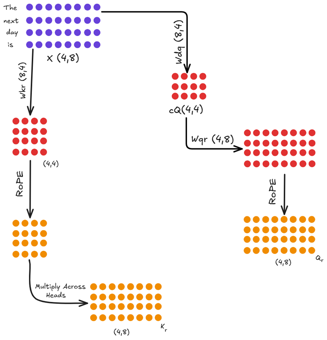
1. Calculating the positional key (Kr):
   • The input $X$ is multiplied by a new weight matrix, $Wkr$.
   • RoPE is then applied to the result.
   • The DeepSeek paper notes a key optimization here: this $Kr$ projection is shared across all heads. The resulting single-head matrix is then repeated or “broadcasted” to match the full number of heads. This saves a significant amount of memory and computation. The final result is the $Kr$ matrix.
2. Calculating the positional query (Qr):
   • The Query path is slightly more complex, mirroring the down-project/up-project structure of the content path to save activation memory.
   • The input $X$ is first down-projected using $Wdq$ to get the same latent query $cQ$ from the content path.
   • This $cQ$ is then multiplied by a new weight matrix, $Wqr$.
   • Finally, RoPE is applied to this result to produce the final $Qr$ matrix.
   • Unlike the key, the positional queries are not shared. $Wqr$ is a full multi-headed matrix, producing a unique positional query for each head.

At the end of this path, we have two new matrices, $Qr$ and $Kr$, which contain pure, relative positional information. The only part that needs to be cached for this path is the shared, rotated key matrix, $Kr$.

The positional query matrix, $Qr$, does not need to be cached. This follows the same fundamental principle we established for standard KV caching in chapter 2: during autoregressive generation, we only ever need the query information for the single, most recent token to predict the next one. Since the query vector for the current token must always be computed fresh, there is no benefit to caching the query vectors from past tokens.

3.14.2 Combining the paths to calculate final attention

Now that we have the outputs from both parallel paths, we can combine them to calculate the final attention scores. The full Query matrix $Q$ is the concatenation of the content query $Qc$ and the positional query $Qr$. The full Key matrix $K$ is the concatenation of $Kc$ and $Kr$.

The final attention score is the dot product of these two combined matrices.

Figure 3.30 The final attention score calculation. The scores are the sum of the content-based scores and the position-based scores.

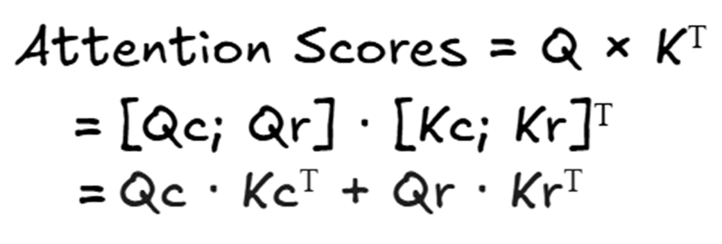
As the mathematical identity in figure 3.30 shows, this is equivalent to calculating the attention scores for each path separately and then adding them together:

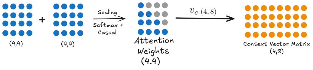
This is the beauty of the decoupled design. We calculate the position-agnostic, cache-friendly content scores and add them to the position-dependent, RoPE-infused scores. Finally, these combined scores are used to create the attention weights, which are then multiplied by the content-only Value matrix to produce the final context vector.

Figure 3.31 The final step. The combined attention scores are processed and multiplied by the content-based Value matrix (Vc) to produce the final output.

This elegant, decoupled system successfully solves the incompatibility problem. It allows the absorption trick to be used on the content-heavy part of the calculation (the $Qc * Kc^T$ term) while still incorporating the full power of RoPE in a separate, specialized path. It truly achieves the best of both worlds.

3.14.3 The cost of decoupling: A trade-off between memory and computation

The Decoupled RoPE architecture is a brilliant solution, but it’s not entirely “free.” By creating a separate, parallel path for positional information, we have introduced new computations and new weight matrices. Let’s analyze the costs and trade-offs of this design.

The new computational cost

In a standard MLA or even the “pure” MLA we designed, the core computation for attention scores is a single large matrix multiplication: $Q * K^T$.

In the decoupled architecture, we now perform two separate matrix multiplications that are added together:

1. Qc @ Kc.T (the content scores)
2. Qr @ Kr.T (the positional scores)

Furthermore, we’ve added new projection steps to generate $Qr$ and $Kr$ in the first place. This means that for each token, the model is performing more floating-point operations (FLOPs) than it would in a simpler architecture. This is a deliberate trade-off: we are accepting a slight increase in computational cost to gain a massive reduction in memory cost.

Why is this a good trade-off?

In modern, large-scale LLMs, the primary bottleneck during long-context inference is almost always memory bandwidth, not raw computation. The process of loading the massive KV cache from the GPU’s high-bandwidth memory (HBM) into the much faster on-chip SRAM for computation is the slowest part of the process.

• Standard MHA: Has fewer computations but is severely bottlenecked by the time it takes to read its enormous 400 GB KV cache.
• Decoupled MLA+RoPE: Has slightly more computations but is much faster overall because it only needs to read a tiny ~7 GB cache.

The time saved by avoiding the memory bottleneck far outweighs the extra time spent on the additional matrix multiplications. DeepSeek made a calculated engineering decision to trade a resource they had in abundance (compute) to save a resource that was critically scarce (memory bandwidth).

The new parameter cost

The decoupled path also introduces new learnable weight matrices: $Wkr$ and $Wqr$. This means the total parameter count of the model increases slightly. However, these matrices are relatively small compared to the enormous feed-forward networks in each Transformer block. The increase in the model’s overall size is negligible, but it’s a factor to consider.

In summary, decoupled architecture isn’t magic, it’s a masterful piece of engineering that makes a highly favorable trade-off. It strategically increases the amount of computation and the number of parameters by a small amount to solve the much larger, more critical problem of memory bandwidth, ultimately leading to a faster and more efficient model.

3.14.4 The new inference loop in action: What happens when a new token arrives

Now that we understand the complete decoupled architecture, let’s trace the full, end-to-end journey of a single new token. This will solidify our understanding of how MLA and RoPE work together in an efficient, autoregressive loop.

Imagine our model has already processed the sequence “The next day is” and has just generated the token “bright.” The input for this inference step is only the embedding for “bright,” which we’ll call $X_bright$. Our goal is to use this single new token to predict the next one.

The process happens in two parallel paths: the Content Path and the Position Path, which are then combined.

The content path: Leveraging the absorption trick

This path is responsible for calculating the content-based attention scores. It uses the pure MLA mechanism, which is highly efficient thanks to the absorption trick and the latent KV cache.

Figure 3.32 The computational flow for the content-based attention score.

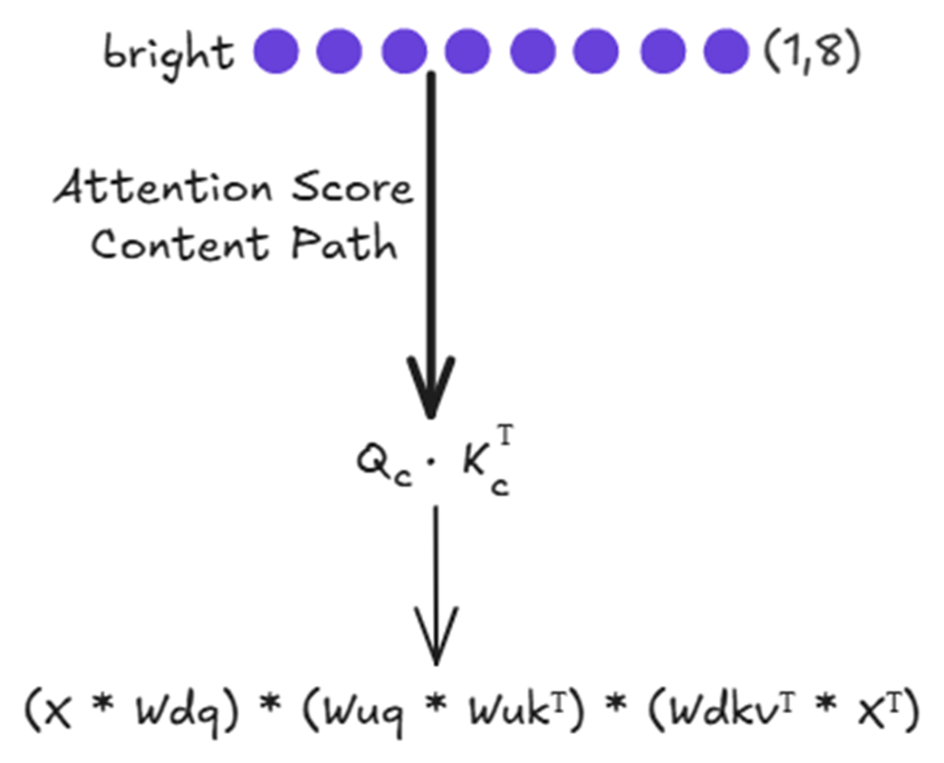
As shown in figure 3.32, the final attention score $q_c * k_c^T$ is calculated from a series of matrix multiplications. Let’s break down how this works for our new token, “bright.”

The first thing we need is the query for our new token. Because of the absorption trick, we don’t just compute a standard query. Instead, we compute an “absorbed query” that already includes the Key up-projection matrix.

Figure 3.33 This single multiplication gives us the query part we need for the content score.

Next, we need to update our historical context. We take the input embedding for our new token, $X_bright$, and compute its compressed representation.

Figure 3.34 Updating the Latent KV Cache. The new token’s embedding is down-projected to create a new latent vector, which is then appended to the existing cache.

As shown in figure 3.34:

1. $X_bright$ (shape 1, 8) is multiplied by the down-projector $Wdkv$ (shape 8, 4).
2. This produces the new latent vector for “bright” (shape 1, 4).
3. This new vector is appended to the existing Latent KV Cache (which was shape 4, 4), resulting in an Updated KV Cache of shape (5, 4).

This updated cache is the only piece of historical information we need for the entire content path. Now we can calculate the content score. We multiply our “Absorbed Content Query” by the transpose of our Updated KV Cache. This gives us the final content-based attention scores for the token “bright.”

The position path: Injecting rotational information

Running in parallel to the content path is the specialized path for handling positional information. Its goal is to compute the position-based attention scores using RoPE.

Figure 3.35 The computational flow for the position-based attention score.

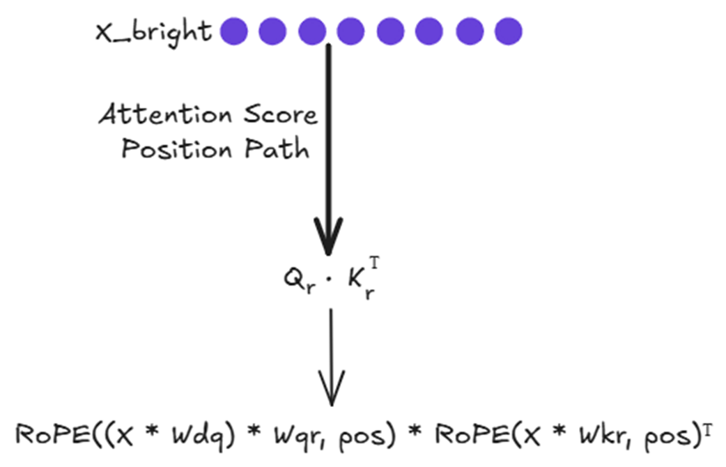
As shown in figure 3.35, the final positional score $q_r * k_r^T$ is also the result of a series of transformations. You might recall that the position-dependent nature of RoPE was what broke the absorption trick in our initial attempt to combine it with MLA. So why is it not a problem here?

The answer lies in the decoupled design. The Position Path operates in parallel and does not rely on the $cKV$ latent cache from the Content Path. Since there is no “absorption trick” to break in this specialized path, we are free to apply RoPE as needed to infuse the $Qr$ and $Kr$ vectors with positional information.

Let’s break down how this works for our new token, “bright”, which is at position 4 (assuming 0-indexing).

First, we need to create the query vector that will be encoded with positional information. This involves a down-projection and an up-projection, just like the content query, to save activation memory.

Next, we need the Key matrix for the positional path. This involves computing the new key for “bright” and appending it to the cached keys from previous tokens. With the fresh $Qr$ and the updated $Kr$ Cache, we can now compute the final positional attention scores by taking their dot product: $Qr * Kr_cache^T$.

3.15 Quantifying the gains: The final cache memory comparison

The multi-step, decoupled process of the fused MLA-RoPE architecture is a masterpiece of engineering. But what does it achieve in practice? Let’s quantify the two main benefits we set out to achieve: a dramatic reduction in cache size and the preservation of the model’s expressive performance.

In the previous chapter, we established the formulas for the memory cost of MHA, MQA, and GQA. Now, we can define the final formula for our advanced MLA with Decoupled RoPE.

The crucial insight is that at each step, we only need to store two things in memory:

• The Latent KV Cache: This stores the compressed content information for all past tokens. Its dimension per token is $d_latent$.
• The Decoupled Key Cache: This stores the rotated positional information for all past tokens. Its dimension per token is $d_rope$.

Therefore, the new formula for the size of the cache is:

Let’s break this down:

• $l$ (layers), $b$ (batch size), $s$ (sequence length), and 2 (bytes per parameter) are the same as before.
• The $(d_latent + d_rope)$ term replaces the $g * h$ from GQA or the $n * h$ from MHA.
• The * 2 factor that previously accounted for storing two separate matrices (one for Keys and one for Values) is gone. In this new architecture, we are caching specialized, combined representations ($d_latent$ for content and $d_rope$ for the positional key), not separate $K$ and $V$ matrices.

Let’s plug in the numbers for a model at the scale of DeepSeek-V2, where $n=128$ and $h=128$:

• MHA Cache Dimension: $2 * 128 * 128 = 32,768$
• MLA+RoPE Cache Dimension: In the DeepSeek paper, $d_latent$ is $4 * h = 512$, and $d_rope$ is $h / 2 = 64$. The total is $512 + 64 = 576$.

The final reduction in the size of the cached data is: $32,768 / 576 \approx 57$ times.

This is an incredible result. By decoupling content and position and using a compressed latent cache, the MLA+RoPE architecture reduces the memory footprint of the KV cache by nearly two orders of magnitude compared to standard MHA. The theoretical 400 GB cache we calculated collapses to a much more manageable ~7 GB.

3.16 Building MLA + decoupled RoPE from scratch

We have now covered all the theoretical and mathematical foundations of Multi-Head Latent Attention and Decoupled Rotary Position Embedding. The final step is to translate this knowledge into a functional PyTorch module. The complete, executable code for this chapter can be found in the book’s official GitHub repository. We highly recommend having it open to follow along with the implementation:

https://github.com/VizuaraAI/DeepSeek-From-Scratch/tree/main/ch03

Our implementation will construct the DeepSeekAttention module, which contains the entire decoupled architecture. Before we write the code, let’s look at a complete visual blueprint of the module’s forward pass in figure 3.36.

Figure 3.36 A detailed flowchart of the DeepSeekAttention module. The input tensor x is processed through two parallel streams: the blue Content Path, which uses pure MLA for cache efficiency, and the purple Position Path, which applies RoPE. The two cached tensors, c_kv and k_r, are highlighted with key icons. The outputs are combined to produce the final context vector.

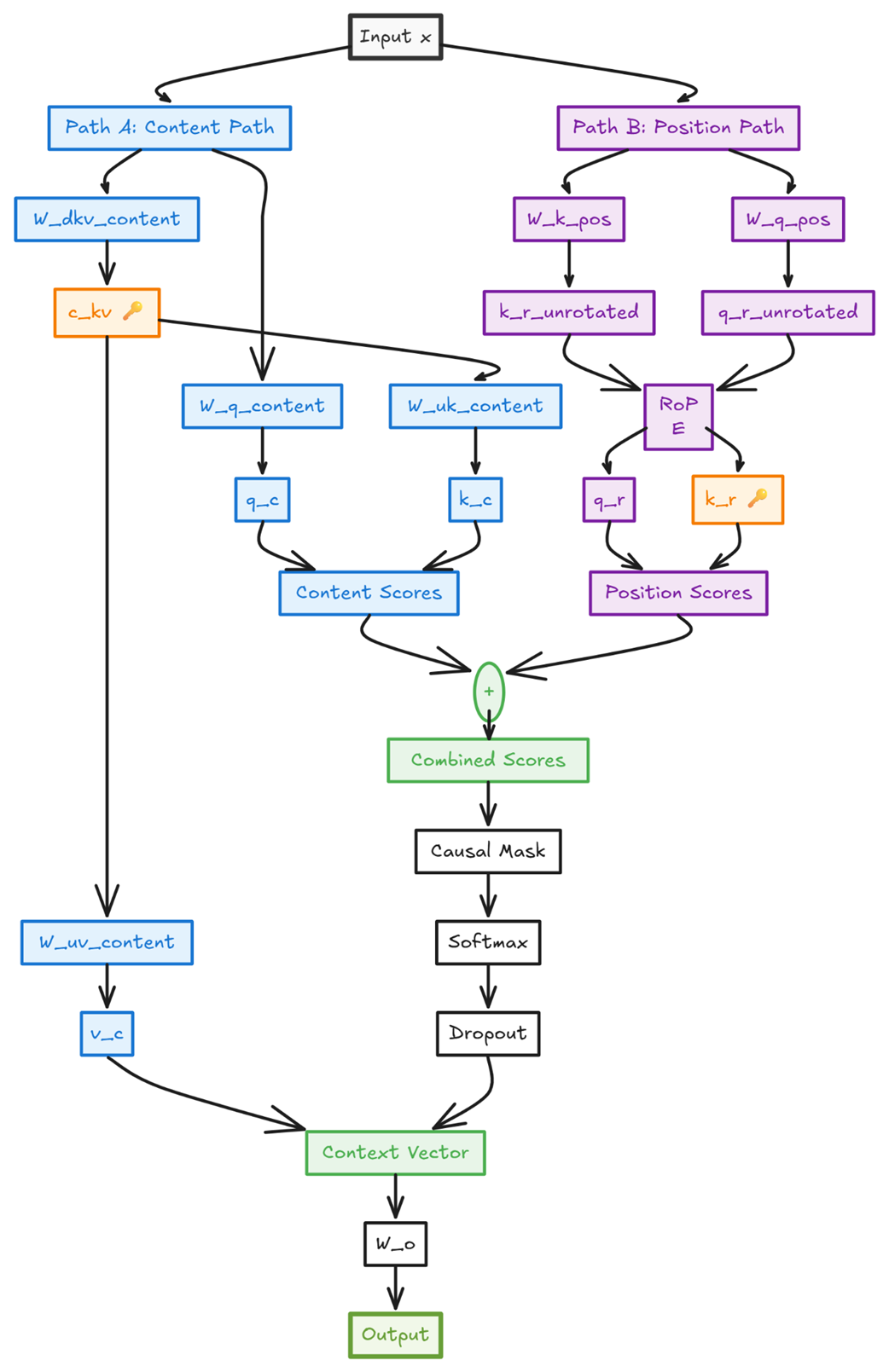
This diagram is a direct map of the code we are about to build. It clearly shows the two parallel pathways:

1. Path A: The Content Path: This stream is responsible for understanding the semantic content of the tokens. It uses the pure MLA architecture, creating the compressed latent tensor c_kv which is the only content-based value we need to cache. It also produces the content-based Query (q_c), Key (k_c), and Value (v_c) matrices.
2. Path B: The Position Path: This stream is dedicated to understanding the relative positions of tokens. It creates specialized Key (k_rope) and Query (q_rope) vectors, which are then infused with positional information by the RoPE module. The resulting rotated key, k_r, is the second value we cache.

The attention scores from these two paths are added together. The resulting attention weights are then applied to the content-only Value (v_c) to produce the final context vector.

Breaking down a complex architecture like this into smaller, manageable pieces is a key engineering skill. We will follow this principle by constructing our DeepSeekAttention module in stages, starting with the self-contained RoPE helper class.

Part 1: The RotaryPositionalEncoding Helper Class

Before we can build the main attention module, we need a way to implement RoPE. It’s a self-contained concept, making it the perfect candidate for our first code snippet. We will present the RotaryPositionalEncoding class in its entirety because it’s a single, cohesive unit.

Listing 3.2 The RotaryPositionalEncoding Helper Module

import torch
import torch.nn as nn
 
class RotaryPositionalEncoding(nn.Module):
    def __init__(self, d_head, max_seq_len=2048):
        super().__init__()
        # Precomputes the base frequencies (theta) for the rotations, one for each pair of dimensions in the head.
        theta = 1.0 / (10000 ** (
        torch.arange(0, d_head, 2).float()
        / d_head))
        self.register_buffer('theta', theta)
        
        # Precomputes the full rotational matrices (freqs_cis) for all positions up to max_seq_len using the complex number representation cos(theta) + i*sin(theta).
        positions = torch.arange(max_seq_len).unsqueeze(1)
        freqs = positions * self.theta.unsqueeze(0)
        
        self.register_buffer('freqs_cis', 
        torch.polar(torch.ones_like(freqs),
        freqs))
 
    def forward(self, x):
        seq_len = x.shape[2]
        # Reshapes the input vector by pairing adjacent dimensions and casting them as complex numbers, ready for rotation.
        x_complex = x.float().reshape(*x.shape[:-1], -1, 2)
        x_complex = torch.view_as_complex(x_complex)
        
        freqs_cis = self.freqs_cis[:seq_len, :].unsqueeze(0).unsqueeze(0)
        
        # Applies the rotation by performing element-wise multiplication in the complex plane. This is the core mathematical operation of RoPE.
        x_rotated = x_complex * freqs_cis
        
        x_rotated = torch.view_as_real(x_rotated)
        x_rotated = x_rotated.flatten(3)
        return x_rotated.type_as(x)

Step 2: Initializing the Main Attention Class

With our RotaryPositionalEncoding module ready, we can now define the main DeepSeekAttention class. The __init__ method is responsible for creating all the learnable weight matrices (nn.Linear layers) and instantiating our RoPE helper.

Notice how the weight matrices are grouped into two distinct sections in the code, mirroring our decoupled architecture. One set is for the content path, which uses the standard MLA projections. The other set is for the position path, which creates the specialized Query and Key vectors that will be infused with positional information via RoPE.

Listing 3.3 Initializing the DeepSeekAttention Module

class DeepSeekAttention(nn.Module):
    def __init__(self, d_model, num_heads, d_latent, d_rope, dropout=0.0):
        super().__init__()
        # ... (asserts and initializations) ...
        self.d_rope = d_rope
        self.num_heads = num_heads
        self.d_head = d_model // num_heads # Assuming d_model is divisible by num_heads
        self.d_model = d_model

        # --- Content Path (Pure MLA) ---
        # The set of projection matrices for the content path, which uses the standard MLA architecture to create a cache-friendly representation of token semantics.
        self.W_q_content = nn.Linear(d_model, d_model)
        self.W_dkv_content = nn.Linear(d_model, d_latent)
        self.W_uk_content = nn.Linear(d_latent, d_model)
        self.W_uv_content = nn.Linear(d_latent, d_model)
        
        # --- Position Path (RoPE Applied) ---
        # The set of projection matrices for the separate position path. These create specialized Query and Key vectors designed to be encoded with positional information.
        self.W_k_pos = nn.Linear(d_model, d_rope * num_heads)
        self.W_q_pos = nn.Linear(d_model, d_rope * num_heads)
        
        # Instantiates the RoPE helper module, which will be used to apply the positional rotations.
        self.rope = RotaryPositionalEncoding(d_rope)
        
        # --- Final Output Projection ---
        self.W_o = nn.Linear(d_model, d_model)
        self.dropout = nn.Dropout(dropout)
        # ... (mask initialization) ...
        self.register_buffer('mask', torch.triu(torch.ones(1, 1, 1024, 1024), diagonal=1).bool())

Step 3: The Forward Pass - Combining Content and Position

The forward method handles the entire decoupled attention calculation. It takes the input tensor x and passes it through both the content and position paths simultaneously to compute two separate attention score matrices. These are then added together to form the final scores, which are used to generate the context vector.

This implementation is a direct translation of the architecture we derived. It keeps the cache-friendly “absorption trick” alive for the content path while cleanly integrating the position-dependent rotations in a separate, parallel stream.

Listing 3.4 The forward Method of DeepSeekAttention

    def forward(self, x):
        batch_size, seq_len, _ = x.shape
 
        # --- Content Path Calculation ---
        q_c = self.W_q_content(x).view(
                 batch_size, seq_len, self.num_heads, self.d_head
             ).transpose(1, 2)
        c_kv = self.W_dkv_content(x)
        k_c = self.W_uk_content(c_kv).view(
                 batch_size, seq_len, self.num_heads, self.d_head
             ).transpose(1, 2)
        v_c = self.W_uv_content(c_kv).view(
                 batch_size, seq_len, self.num_heads, self.d_head
             ).transpose(1, 2)
        
        # --- Position Path Calculation ---
        q_r_unrotated = self.W_q_pos(x).view(
                 batch_size, seq_len, self.num_heads, self.d_rope
             ).transpose(1, 2)
        k_r_unrotated = self.W_k_pos(x).view(
                 batch_size, seq_len, self.num_heads, self.d_rope
             ).transpose(1, 2)
 
        # Applies Rotary Positional Encoding to the unrotated positional Query and Key vectors. This is where positional information is injected.
        q_r = self.rope(q_r_unrotated)
        k_r = self.rope(k_r_unrotated)
        
        # --- Combining Paths for Final Attention Score ---
        content_scores = (q_c @ k_c.transpose(-2, -1)) / \
                 (self.d_head ** 0.5)
        position_scores = (q_r @ k_r.transpose(-2, -1)) / \
                 (self.d_rope ** 0.5)
        
        # The final attention score is the sum of the content-based scores and the position-based scores, elegantly combining the two parallel paths.
        attn_scores = content_scores + position_scores
        
        # --- Final Steps (Masking, Softmax, Output) ---
        attn_scores = attn_scores.masked_fill(
                 self.mask[:, :, :seq_len, :seq_len], float('-inf'))
            
        attn_weights = torch.softmax(attn_scores, dim=-1)
        attn_weights = self.dropout(attn_weights)
        
        context_vector = (attn_weights @ v_c).transpose(1, 2) \
                 .contiguous().view(batch_size, seq_len, self.d_model)
            
        output = self.W_o(context_vector)
        return output

With this final snippet, we have constructed a complete, from-scratch implementation of the DeepSeekAttention module. This single class encapsulates a series of advanced techniques:

• A memory-efficient content pathway using Multi-Head Latent Attention.
• A separate, specialized position pathway for handling relative positions.
• Clean integration of Rotary Positional Encoding where it is most effective.
• A decoupled fusion of these two pathways through simple addition.

This architecture masterfully resolves the inherent conflict between the position-agnostic caching of MLA and the position-dependent nature of RoPE. By trading a slight increase in computational cost for a massive reduction in memory bandwidth requirements, this design achieves the best of both worlds, enabling efficient and powerful long-context inference.

3.17 The Payoff: An Empirical Head-to-Head Comparison

Having explored the theoretical and mathematical underpinnings of Multi-Head Latent Attention and its fusion with Decoupled RoPE, it’s time to put our knowledge to the test. Theory is one thing, but empirical results provide the final verdict. The central promise of MLA is to break the painful trade-off between the high performance of MHA and the memory efficiency of its leaner cousins, MQA and GQA. Does it truly deliver the best of both worlds?

To answer this, we conducted a head-to-head comparison by building and training four models from scratch. Each model uses a different attention mechanism, but all other hyperparameters from model size and dataset to the number of training iterations are held constant to ensure a fair and direct comparison. This experiment will allow us to move beyond theory and quantify the real-world impact of DeepSeek’s architectural innovations.

The code used to run this experiment and generate the following results is available for you to explore and replicate in the book’s GitHub repository.

Bonus Code Link: https://github.com/VizuaraAI/DeepSeek-From-Scratch/tree/main/ch03/02-bonus-code

To properly evaluate the trade-offs, we will train and benchmark four distinct attention architectures:

1. Multi-Head Attention (MHA): Our baseline for maximum performance. Each head has its own unique Query, Key, and Value projections, foregoing the highest efficiency at the cost of a large KV cache.
2. Multi-Query Attention (MQA): The first efficiency-focused variant. All heads share a single Key and Value projection, drastically reducing the KV cache size but potentially limiting the model’s learning capacity.
3. Grouped-Query Attention (GQA): A compromise between MHA and MQA. Query heads are divided into groups, with each group sharing a common Key and Value projection. This offers a middle ground in both performance and efficiency.
4. Multi-Head Latent Attention (MLA): The DeepSeek innovation. As we’ve seen, it uses a compressed latent cache and decoupled RoPE to aim for the performance of MHA with the memory footprint closer to MQA/GQA.

Before we begin the training process, it’s crucial to confirm that our models are of a comparable size. A significant difference in the total number of learnable parameters would make for an unfair comparison. The table below shows the parameter counts for each of our four model variants, demonstrating that they are all within a very similar range.

Table 3.1 Parameters of model variants

Attention Type	Total Parameters
Multi-Head Attention (MHA)	17,653,248
Grouped-Query Attention (GQA)	16,965,120
Multi-Query Attention (MQA)	17,260,032
Multi-Head-Latent Attention (MLA)	17,391,104

The total number of learnable parameters is nearly identical across all four architectures, ensuring a fair comparison of their performance and efficiency. The minor differences come from the unique projection matrices required by each attention mechanism.

Our first objective is to answer the most critical question: does MLA’s memory-saving design compromise its learning performance? A lower validation loss indicates better generalization to unseen data, which is our primary measure of a model’s effectiveness. The plot in figure 3.37 tracks the validation loss for all four models over 5,000 training iterations.

Figure 3.37 A comparison of the validation loss curves for the four attention mechanisms. The MHA and MLA models achieve a consistently lower final loss than their MQA and GQA counterparts, indicating superior learning. Both models were trained for 5,000 iterations.

The learning curves reveal an edge. While all four models successfully learn to process the TinyStories dataset, their performance diverges. The MHA and MLA curves track each other closely, achieving the lowest validation loss and demonstrating the strongest learning capability. MQA, as expected, lags slightly behind due to its reduced expressivity, with GQA occupying the middle ground. This plot provides our first piece of powerful evidence: the MLA architecture does not sacrifice performance. It learns just as effectively as the full, resource-intensive MHA model, successfully preserving the expressive power of having unique, multi-headed projections.

Table 3.2 Comparison of attention types

Attention Type	Best Validation Loss	KV Cache Memory Size (MB)	Best Validation Perplexity
MHA	2.3721	48.00	10.72
MQA	2.4080	6.00	11.11
GQA	2.3776	24.00	10.78
MLA	2.3089	12.00	10.06

The results in table 3.2 are definitive. While the validation perplexity confirms what we saw in the learning curves—that MLA achieves the best performance (10.06), closely followed by MHA (10.72)—the KV Cache size column reveals the other half of the story. MLA dramatically reduces the memory footprint by 4x compared to MHA (12.00 MB vs. 48.00 MB), validating the core motivation behind the latent cache architecture.

This head-to-head experiment provides a clear verdict. By decoupling the content and position pathways and leveraging a compressed latent cache, the DeepSeek architecture successfully breaks the performance-memory trade-off. The result is an attention mechanism that is not only powerful but also remarkably efficient, providing a solid foundation for the scalable and intelligent models we aim to build. We will turn to the other key component of the Transformer layer in chapter 4. We will explore how Mixture-of-Experts (MoE) replaces the standard Feed-Forward Network to unlock another dimension of efficient scaling and we will also see DeepSeek Innovations.

3.18 Summary

• Multi-Head Latent Attention (MLA) breaks the performance-memory trade-off by caching a compressed latent representation of Keys and Values, which is then decompressed on-the-fly to reconstruct unique, full-sized matrices for each head during the attention calculation.
• Applying positional information by adding it to the initial token embeddings pollutes their semantic meaning before they are processed by the attention mechanism.
• Rotary Positional Encoding (RoPE) solves this by rotating the Query and Key vectors directly within the attention block, which injects positional information later in the process and preserves the vectors’ original learned magnitudes.
• The efficiency of MLA depends on a mathematical “absorption trick” that requires position-agnostic weights, which is fundamentally incompatible with the position-dependent transformations of standard RoPE.
• The Decoupled RoPE architecture resolves this conflict by separating attention into two parallel streams: a content path that uses a cache-efficient MLA, and a position path that handles RoPE. The final attention scores are the sum of the outputs from both paths.