4 Mixture-of-Experts (MoE) in DeepSeek: Scaling intelligence efficiently

This chapter covers

• Mixture of Experts (MoE) and how sparsity enables efficient scaling
• A hands-on, mathematical walkthrough of the MoE layer
• DeepSeek’s advanced solutions for load balancing

The idea of Mixture of Experts (MoE) is not new; its roots trace back to a seminal 1991 paper on adaptive expert systems. However, its application to large-scale language models is a more recent development, and one that DeepSeek has pushed to its notable limits. While other models like Mistral’s Mixtral brought MoE into the mainstream for LLMs, DeepSeek built upon this foundation, introducing novel tricks and techniques of its own.

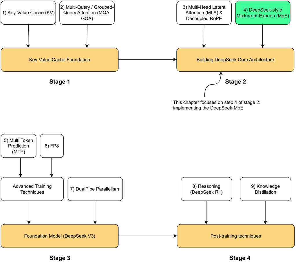
Now let’s open the black box of this mechanism. As illustrated in Figure 4.1, our roadmap will cover:

1. The core intuition behind MoE and the concept of sparsity.
2. A detailed, mathematical, hands-on demonstration of how the MoE mechanism is implemented.
3. An exploration of the critical challenge of “load balancing” and the standard solutions.
4. A deep dive into the specific innovations DeepSeek introduced in their MoE architecture, from shared experts to their auxiliary-loss-free balancing.
5. Finally, we will put it all together by coding a complete, functional MoE language model from scratch.

Let’s begin by understanding how MoE fits into the Transformer architecture and the core idea that makes it so powerful.

4.1 The intuition behind mixture of experts

To understand Mixture of Experts, we must first look at the component it replaces within the standard Transformer block: the Feed-Forward Network (FFN). The FFN acts as the primary processing unit within each Transformer layer, a dense neural network that accounts for the majority of the model’s parameters and its computational workload. This change marks a genuine revolution in design. Instead of relying on one massive, all-purpose neural network, we now substitute it with a diverse number of smaller, specialized neural networks each an “expert” in its own right. MoE allows models to grow far larger and more knowledgeable without a proportional increase in computational cost.

4.1.1 The problem with dense FFNs in transformer: High parameter count and computational cost

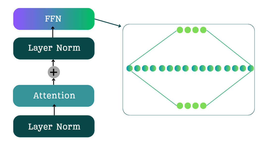
As we know following the multi-head attention layer and layer norm, the resulting context vectors are processed by a Feed-Forward Network (FFN), the architecture of which is depicted in Figure 4.2. The FFN consists of a two-layer neural network that implements an “expansion-contraction” sequence. As Figure 4.2 illustrates, the first linear layer expands the embedding dimension (e.g., by a factor of 4), while the second linear layer contracts it back to its original size. This design is critical for the model’s performance, as the expanded intermediate layer provides a richer, higher-dimensional space for the model to capture complex patterns before the output is passed to the subsequent block.

However, this FFN is dense. This means that for every single input token, all of the millions of parameters in the FFN are activated and used in the computation. This has two major consequences:

1. High Training Cost: The large number of parameters in the FFNs across all Transformer blocks accounts for a significant portion of the model’s total training time.
2. High Inference Cost: Similarly, during inference, these dense computations contribute significantly to the latency of generating each new token.

4.1.2 The sparsity solution: Activating only a subset of experts per token

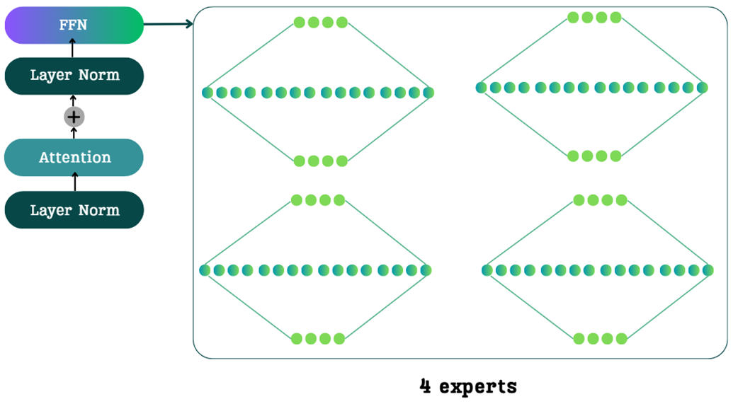
The core idea of Mixture of Experts is to replace the single, large, dense FFN with a collection of multiple, smaller FFNs, which we call “experts.” The traditional FFN is a single, dense network. In an MoE architecture, this single block is replaced by a set of parallel expert networks, as shown in Figure 4.3.

You might think that replacing one network with four would quadruple the computational cost, but this is where the magic of MoE comes in, driven by a single concept: sparsity.

Sparsity: In an MoE model, for any given input token, only a small subset of the total experts is activated. The rest remain dormant or inactive.

For example, in the 4-expert model shown in Figure 4.3, a token might be routed to only one or two of them. The other experts are not used for that specific token, meaning their parameters are not loaded and their computations are not performed.

This is the source of MoE’s incredible efficiency. We get the benefit of having a huge number of total parameters (the sum of all experts), but the computational cost for any single token is very low, as we only activate a small fraction of them. This allows us to build models that are vastly more knowledgeable (more total parameters) without a proportional increase in the cost of training or inference.

4.1.3 Expert specialization: The “why” behind sparsity

The concept of sparsity activating only a few experts per token is what makes MoE efficient. But why does this work? Why can we get away with ignoring most of the experts? The answer lies in expert specialization.

During the massive pre-training process, each expert network learns to become highly specialized in handling specific types of information or performing particular tasks. Instead of one giant, generalist FFN that must know how to do everything, we have a committee of specialists.

This specialization was proven quantitatively in the 2022 paper “ST-MoE: Designing Stable and Transferable Sparse Expert Models,” (https://arxiv.org/pdf/2202.08906) which analyzed what different experts in a trained model had learned to do. The results were fascinating and provided a clear window into the mind of an MoE model.

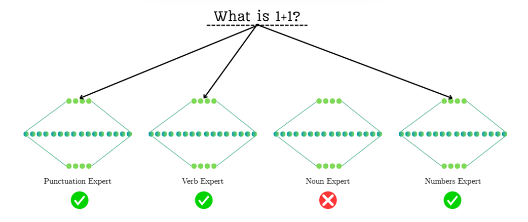
To make this concrete, let’s trace how the model might process the simple question “What is 1+1?”, as illustrated in Figure 4.4. The routing network must look at the incoming tokens and select the most appropriate specialists from its available committee:

• Punctuation Expert: The router first encounters the question mark (?). Having learned to recognize punctuation, it activates the Punctuation Expert. This expert is highly specialized in understanding the role of punctuation marks and how they influence the meaning and structure of a sequence.
• Verb Expert: The token is a common verb. The router, recognizing this, sends the token to the Verb Expert. This specialist has learned the grammatical and semantic patterns associated with actions and states of being, and it is best equipped to handle this part of the input.
• Dormant Experts (e.g., Noun Expert): Notice that the Noun Expert is not activated. Since the query contains no significant nouns, the router intelligently saves computation by keeping this expert dormant. The same would apply to a Proper Noun Expert; since there are no names like “Martin” or “DeepSeek,” that specialist is not needed.
• Domain-Specific Experts: This is where the process becomes even more granular. You might expect the Numbers Expert to be the most critical for handling “1+1”. However, as the diagram shows, the router might have learned that the signals from the question mark and the verb are stronger or more immediately recognizable. In this case, it prioritizes the grammatical experts, leaving the mathematical ones dormant. This highlights the complex and sometimes non-obvious decisions the routing mechanism makes, activating only the experts it deems most relevant for a given token based on its training.

This is the beauty of the MoE design. When an input token arrives, the model doesn’t need to consult its entire knowledge base. It uses a small, efficient routing network (which we will build later) to ask, “Who is the specialist expert for this type of token?” It then sends the token only to the relevant experts.

A token representing a comma does not need to activate the expert that specializes in mathematical verbs. By routing the token only to the punctuation expert, the model saves an enormous amount of computation.

4.2 The mechanics of MoE: A hands-on mathematical walkthrough

Now that we have the core intuition behind Mixture of Experts, it’s time to open the black box and see how it is actually implemented. We will trace the journey of a batch of tokens step-by-step, from the input that enters the MoE block to the final output it produces.

To make the mathematics as clear as possible, we will switch from the previous conceptual example to a new, standard input sequence that is easier to visualize in matrix form. For the remainder of this walkthrough, we will use the input “The next day is.” Our goal is to understand how the model uses sparsity and routing to efficiently combine the knowledge of multiple experts for this sequence.

4.2.1 The goal: Combining multiple expert outputs into one

Let’s start by defining our setup. We have an input matrix of shape (4, 8), representing four tokens (“The”, “next”, “day”, “is”), each with an 8-dimensional embedding. This matrix is the output from the preceding attention layer in the Transformer block.

Let’s assume for our simplified example that our MoE layer contains three separate expert networks (E1, E2, E3), though in a real model this number would be much larger. As we know, each expert is a full Feed-Forward Network. If we were to pass our input matrix through each of these experts, we would get three separate output matrices.

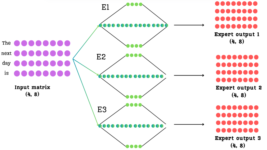
As Figure 4.5 shows, this leaves us with a challenge. We start with one (4, 8) input matrix, but we end up with three (4, 8) output matrices. The Transformer architecture, however, expects only a single matrix to pass to the next layer.

Our entire task in this section is to figure out: How do we intelligently combine these three expert outputs into a single, final output matrix of the same (4, 8) shape? The answer lies in two key concepts we introduced intuitively back in Section 4.1: sparsity and routing.

4.2.2 Sparsity in action: Top-K selection for load balancing

The first step in processing tokens with a Mixture of Experts (MoE) model is selecting which experts to use for each token before merging their outputs. As we’ve discussed, the core efficiency of MoE comes from sparsity: not every token is processed by every expert.

We enforce this by making a simple but powerful decision: for each token, we will only select the top-$k$ most relevant experts. The value of $k$ is a hyperparameter we choose. For our example, we will set $k=2$. This means that out of our three available experts, only two will be activated for any given token.

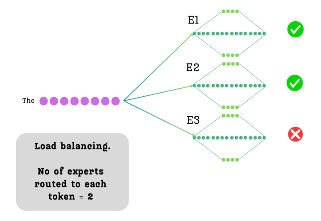
As illustrated in Figure 4.6, when the token “The” is processed, it will only be sent to two of the three experts (in this example, E1 and E2 are selected, while E3 is ignored). This act of selective activation is what prevents the model from having to perform the full computation of all experts for every token.

This immediately raises the next logical question: how does the model decide which two experts to select? And once selected, how does it know how much importance, or weight, to give to each of them? This is the job of the routing mechanism.

4.2.3 The routing mechanism: From input to expert scores

To decide which experts are best suited for each token, the model uses a small, learnable neural network called a router. The router’s job is to look at the input tokens and produce a score for each expert, for each token.

This is implemented as a simple linear layer. We take our Input Matrix and multiply it by a learnable Routing Matrix.

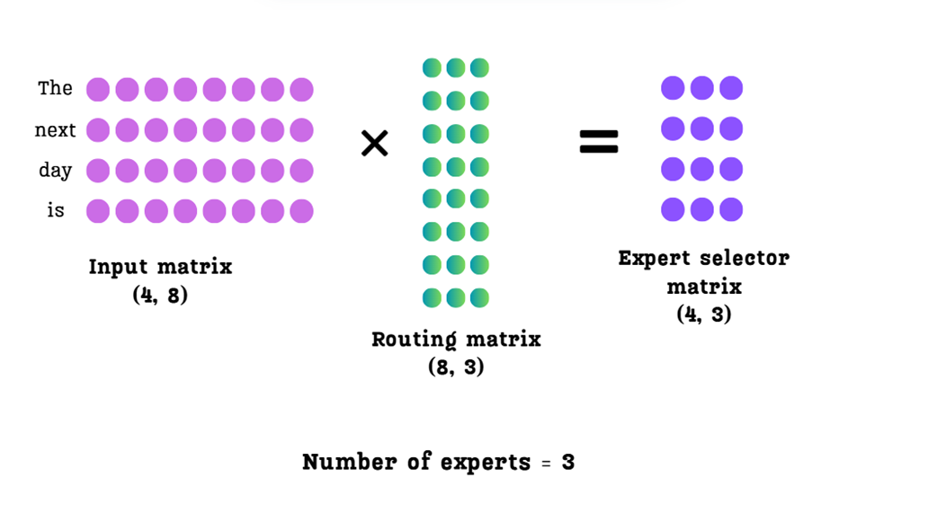
Let’s break down the dimensions shown in Figure 4.7:

• Input Matrix: Shape (4, 8) - four tokens, each with an 8-dimensional embedding.
• Routing Matrix: Shape (8, 3) - the input dimension must match the input matrix (8), and the output dimension is the number of experts we have (3). This is a learned weight matrix.
• Expert Selector Matrix: Shape (4, 3) - the result of the multiplication.

This Expert Selector Matrix (also often called the logits matrix) is the crucial output of the router. Let’s interpret its structure:

• Each row corresponds to one of our input tokens ("The", "next", "day", "is").
• Each column corresponds to one of our experts (E1, E2, E3).
• The value at each position (row, column) is a raw, unnormalized score indicating how suitable that expert is for that token.

For example, the value in the first row, second column is the score for routing the token “The” to Expert 2. Now that we have these scores, we can use them to implement our top-$k$ selection.

4.2.4 From scores to weights: Top-K selection and softmax normalization

We now have our Expert Selector Matrix, which contains the raw scores. Our next task is to use these scores to achieve two goals:

1. Select only the top 2 experts for each token.
2. Convert the scores for those selected experts into a set of weights that sum to 1.

This is a three-step process.

Step A: Select the Top-K Experts

First, for each row (each token), we identify the $k=2$ experts with the highest scores. The scores for all other experts are discarded.

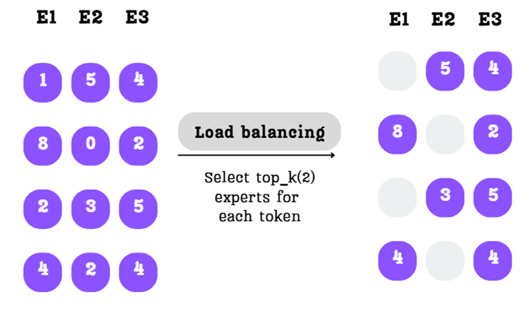
As shown in Figure 4.8, for the first token, the scores 5 and 4 (for E2 and E3) are the highest, so the score 1 (for E1) is masked out. This is repeated for every token, fulfilling our sparsity requirement.

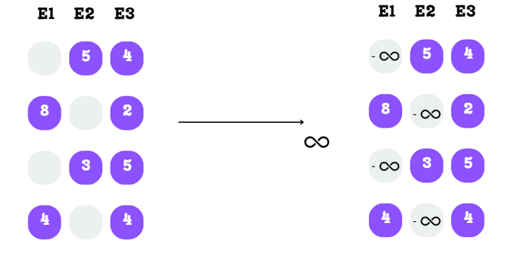
Step B: Masking with Negative Infinity

To mathematically eliminate the non-selected experts, we replace their scores with negative infinity. This might seem like a strange choice, but it’s a clever trick that works perfectly with the softmax function in the next step.

Step C: Applying Softmax

Finally, we apply the softmax function to each row of this new matrix. The softmax function has two properties that are perfect for our needs:

1. It converts any real numbers into a probability distribution where all values are between 0 and 1, and the sum of the values in each row is exactly 1.
2. The exponential function $e^x$ for a very large negative number (like negative infinity) is effectively zero.

As Figure 4.10 shows, applying softmax to our matrix does two things:

• The scores for the non-selected experts (which were negative infinity) become zero.
• The scores for the top-2 selected experts are converted into probabilities that map to 1.

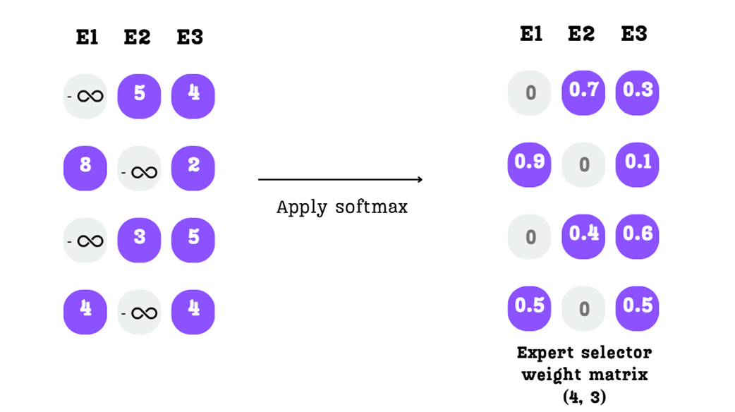
The final output is our Expert Selector Weight Matrix. This matrix now contains all the information we need to combine the expert outputs. For the first token, “The,” it tells us: “Ignore Expert 1, and give 70% of the final output’s weight to Expert 2 and 30% to Expert 4.” We have now answered both of our original questions: which experts to use, and what weight to give them.

4.2.5 The final output: Creating the weighted sum of expert outputs

For each token, we will take the outputs from its selected experts, multiply them by their assigned weights, and add them together. Let’s walk through this for our first token, “The.”

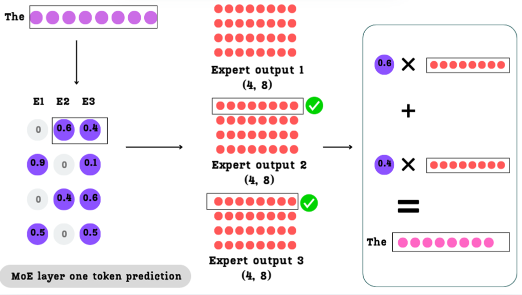
As illustrated in Figure 4.11, the calculation for the token “The” proceeds as follows:

1. Look up the Weights: We look at the first row of our Expert Selector Weight Matrix. It tells us to use Expert 2 with a weight of 0.6 and Expert 3 with a weight of 0.4. Expert 1 has a weight of 0 and will be ignored.
2. Look up the Expert Outputs: We look at the first row (corresponding to the token “The”) of the Expert Output 2 and Expert Output 3 matrices.
3. Perform the Weighted Sum: We perform the following calculation:

(0.6 * OutputVector_The_from_E2) + (0.4 * OutputVector_The_from_E3)

The result is a single (1, 8) vector, which is the final, context-aware output for the token “The.”

This same process is performed in parallel for every token in our input sequence.

• For “next” we would take 0.9 * Output_next_E1 + 0.1 * Output_next_E4.
• For “day” we would take 0.4 * Output_day_E2 + 0.6 * Output_day_E4.
• And so on.

When we stack all of these resulting vectors together, we get our final output matrix.

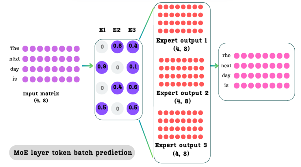
As shown in Figure 4.12, the final output is a single matrix with the same shape as our original input matrix (4, 8). We have successfully replaced the single dense FFN with a sparse mixture of experts. By using the Expert Selector Weight Matrix to perform a weighted sum of only the top-$k$ expert outputs for each token, our new mechanism avoids the expensive computation for all non-selected experts, making it far more computationally efficient than a dense FFN.

4.3 The challenge of balance: Ensuring all experts contribute

We have successfully built a functional Mixture of Experts layer. We have a routing mechanism that uses sparsity (top-k selection) to send each token to a small subset of specialized experts. While this architecture is efficient, it introduces a new and subtle challenge: imbalanced routing.

What happens if the routing network, over the course of training, learns to favor certain experts? This is a common failure mode in MoE training, often driven by a self-reinforcing feedback loop. If a few experts, by chance or data distribution, perform slightly better on early training batches, the router learns to send them more tokens. As they see more tokens, these experts become even more specialized and effective, causing the router to favor them even more heavily in subsequent steps. This feedback loop can quickly lead to a state where some experts get chosen over and over again, while others are rarely, if ever, utilized. This imbalance leads to two significant problems:

• Inefficient Learning: If an expert is never selected, its parameters are never updated. It becomes “dead weight” in the model, contributing nothing to the overall knowledge. We want all of our experts to be contributing members of the committee.
• Performance Degradation: If a few experts become over-utilized “hotspots,” they can become bottlenecks, and the model’s ability to specialize is diminished.

Ideally, we want a balanced MoE model, where, on average, all experts are utilized to a similar degree. To achieve this, several techniques have been developed to encourage the router to distribute the load more evenly. In this section, we will explore the three most important balancing techniques.

4.3.1 Attempt #1: The auxiliary loss

The first and most traditional method for encouraging balance is to add a penalty term to the model’s main training loss. This penalty, called the auxiliary loss, is designed to be high when expert selection is imbalanced and low when it is balanced.

By adding this auxiliary loss to the main next-token prediction loss, we incentivize the model during backpropagation to adjust its routing matrix in a way that leads to a more uniform expert distribution. To understand how this loss is calculated, we must first define a metric for how “important” each expert is.

A. Defining “Expert Importance”

We can measure an expert’s importance by looking at the Expert Selector Weight Matrix.

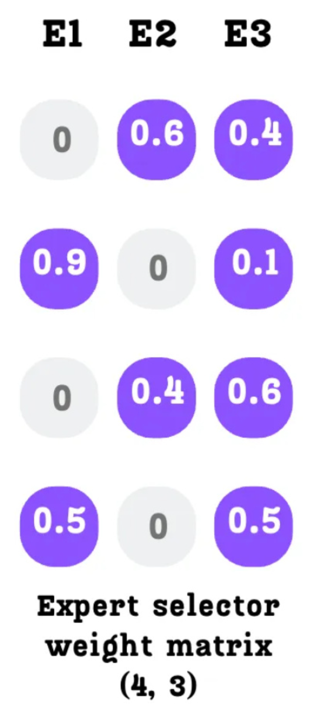
As we know, each column in this matrix corresponds to a specific expert. The values in a column represent the probabilities (or weights) assigned to that expert for each token in the batch. A natural way to measure an expert’s total importance for a given batch is to simply sum the values in its column.

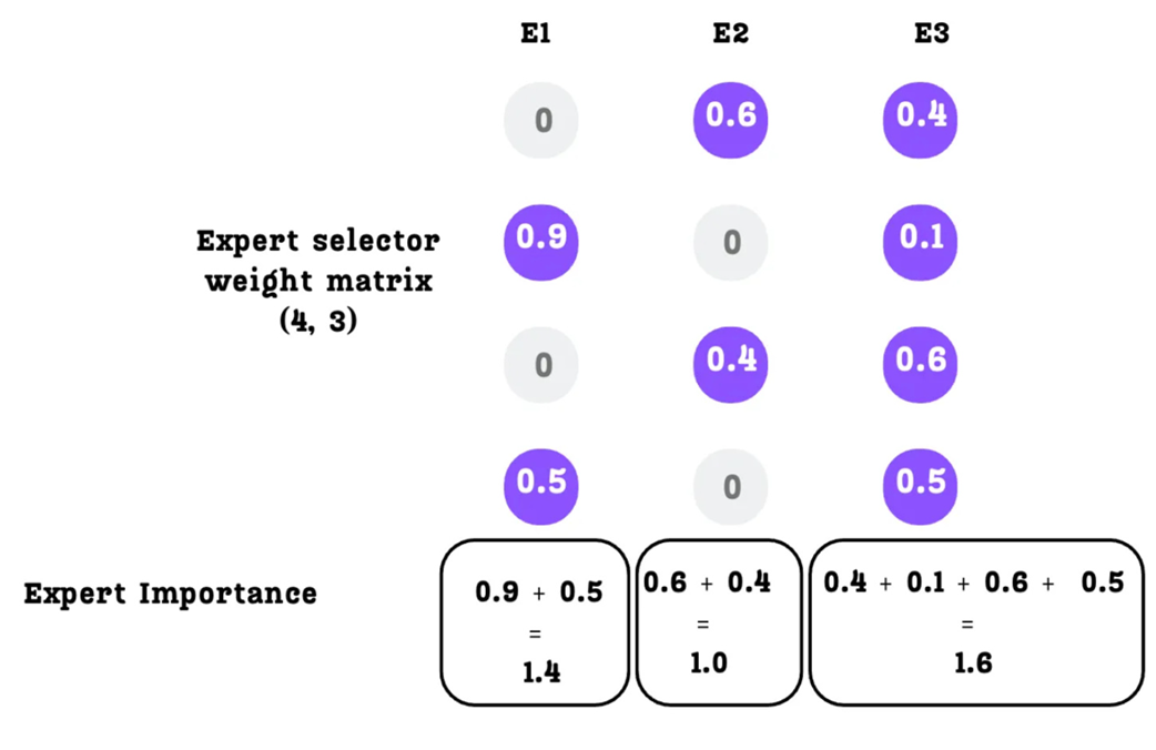
As shown in Figure 4.14, for this specific batch:

• Expert 1 Importance: 0.9 + 0.5 = 1.4
• Expert 2 Importance: 0.6 + 0.4 = 1.0
• Expert 3 Importance: 0.4 + 0.1 + 0.6 + 0.5 = 1.6

These values clearly show an imbalance. Expert 3 is being utilized the most, while Expert 2 is the least utilized. Our goal is to make these importance scores as similar as possible.

B. Calculating the Auxiliary Loss

We want to penalize the model when there is a large variation in the expert importance scores. A standard statistical measure for variation in a set of numbers is the Coefficient of Variation (CV). It’s defined as the ratio of the standard deviation (σ) to the mean (μ):

\[CV = \frac{\sigma}{\mu}\]

The CV is a normalized measure of dispersion. A high CV means the values are very spread out (imbalanced), while a low CV means the values are very close to each other (balanced). Our goal is to make the model learn a routing strategy that results in a low CV for the expert importance scores.

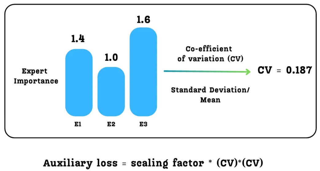
As illustrated in Figure 4.15, we take our three importance scores (1.4, 1.0, 1.6), calculate their CV (which turns out to be 0.187 in this case), and then plug this into our auxiliary loss formula:

\[\text{AuxLoss} = \lambda \cdot CV(\text{ImportanceScores})^2\]

Here, $\lambda$ (lambda) is a scaling factor, a hyperparameter that we choose to control how much we care about this balancing loss compared to the main next-token prediction loss.

This Auxiliary Loss is then added directly to the main training loss. During backpropagation, the model will now receive gradients from two sources: one telling it to get better at predicting the next token, and another telling it to make the expert importance scores more uniform. This pushes the routing function towards a more balanced distribution.

However, as we will see next, simply balancing “importance” is not the full story. It doesn’t necessarily guarantee that the actual number of tokens sent to each expert is balanced, which leads us to a more sophisticated technique.

4.3.2 Attempt #2: The load balancing loss

While the auxiliary loss helps encourage a balance of importance, it has a subtle but critical flaw: assigning equal importance to experts does not necessarily lead to uniform token routing.

This is a key concept. An expert’s “importance” is the sum of probabilities, while its “load” is the actual number of tokens it processes. These two things are not the same. Let’s consider a simple, illustrative example.

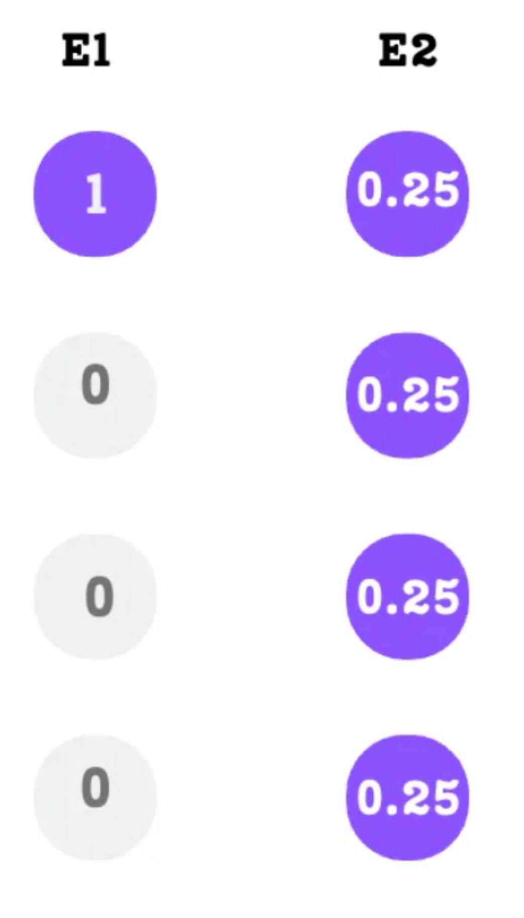
As shown in Figure 4.16, we have a scenario with two experts:

• Expert 1: Receives a single token with a very high probability (1.0). Its total importance is 1.0.
• Expert 2: Receives four different tokens, but each with a low probability (0.25). Its total importance is 0.25 * 4 = 1.0.

Both experts have the same importance score, so the auxiliary loss would be zero and it would see this situation as perfectly balanced. However, the actual workload is extremely imbalanced. Expert 2 is processing four times as many tokens as Expert 1. This can still lead to memory issues and inefficient use of the expert networks.

To solve this, we need a loss function that considers not just the probabilities, but also the actual number of tokens dispatched to each expert. This is the Load Balancing Loss.

The formula for this loss, which we aim to minimize, is defined as the product of the fraction of tokens dispatched to an expert and the probability of the router choosing that expert, summed over all experts. This is then scaled by the number of experts (N) and a hyperparameter $\lambda$:

\[\text{LoadBalancingLoss} = \lambda \cdot N \cdot \sum_{i=1}^{N} (f_i \cdot p_i)\]

To understand how minimizing this value encourages balance, we need to deconstruct its two crucial, per-expert components: $f_i$ (the fraction of tokens in the batch dispatched to expert $i$) and $p_i$ (the mean probability of the router choosing expert $i$ across the batch). We will break these down in the following sections.

A. Calculating $p_i$: The Router Probability

The first component, $p_i$, represents the probability that the router will choose a given expert across the entire batch. It’s a measure of the expert’s overall importance. We calculate this by taking the Expert Importance scores we derived in the previous section and normalizing them by the total number of tokens in the batch.

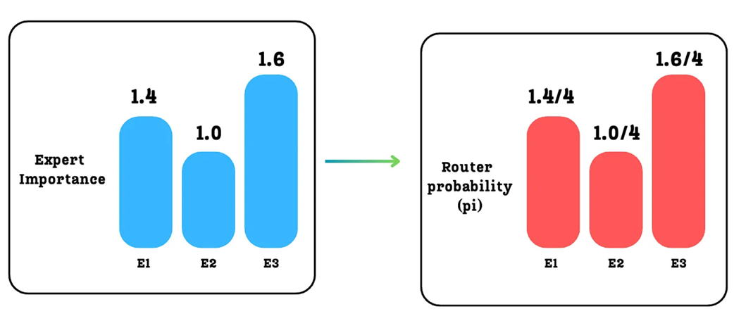
For our example with 4 tokens:

• p1 = ExpertImportance_E1 / 4 = 1.4 / 4 = 0.35
• p2 = ExpertImportance_E2 / 4 = 1.0 / 4 = 0.25
• p3 = ExpertImportance_E3 / 4 = 1.6 / 4 = 0.40

These $p_i$ values give us a normalized view of expert importance.

B. Calculating $f_i$: The Fraction of Tokens Dispatched

The second component, $f_i$, is more direct. It measures the actual fraction of tokens from the batch that are dispatched to each expert after the top-$k$ selection.

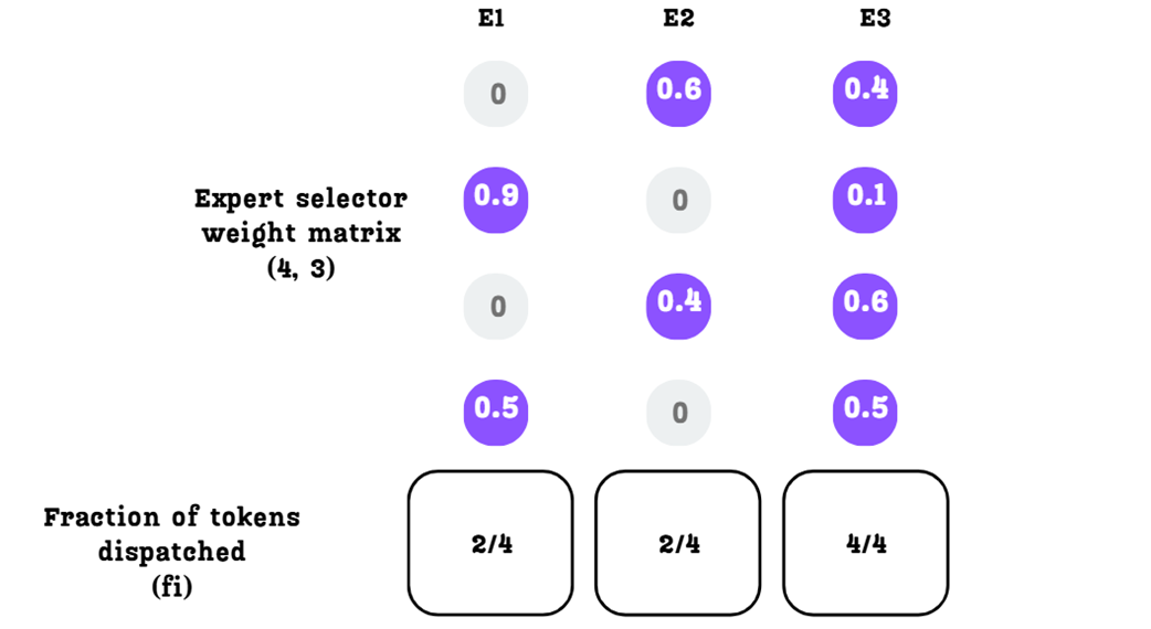
Based on our Expert Selector Weight Matrix and $k=2$ setting:

• Expert 1 is selected for token 2 and token 4. So, f1 = 2/4 = 0.5
• Expert 2 is selected for token 1 and token 4. So, f2 = 2/4 = 0.5
• Expert 3 is selected for tokens 1, 2, 3, and 4. So, f3 = 4/4 = 1.0

C. Minimizing the Loss

By minimizing the product $\sum (f_i \cdot p_i)$, the model is encouraged to align these two distributions. An ideal, perfectly balanced state is one where both $f_i$ and $p_i$ are uniform (e.g., 1/3 for each expert in a 3-expert system). The loss is lowest when the routing is balanced both in terms of probability and in terms of the actual token count. This more sophisticated loss term provides a much stronger signal to the model to avoid situations where one expert becomes a computational bottleneck, leading to more stable and efficient training.

4.3.3 A hard cap: The capacity factor

The Auxiliary and Load Balancing losses are “soft” constraints. They add a penalty to the training objective, encouraging the model to learn a balanced routing strategy over time. However, they don’t strictly prevent situations where, for a given batch, one expert might become temporarily overloaded.

To add a “hard” guardrail, many MoE implementations introduce a concept called the Expert Capacity.

Expert Capacity

A fixed limit on the maximum number of tokens that any single expert is allowed to process within a single batch.

If more tokens are routed to an expert than its capacity allows, the excess tokens are considered “dropped” and do not get processed by that expert for that forward pass.

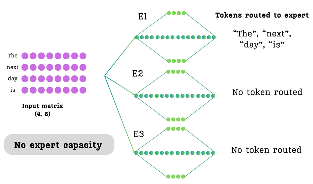
As shown in Figure 4.19, without a capacity limit, it’s possible for the router to send all four tokens to Expert 1, leaving E2 and E3 completely idle for that batch. By setting a capacity of 2, we force the router to distribute the tokens more evenly.

How is Capacity Calculated?

The capacity is typically calculated to be slightly larger than what a perfectly uniform distribution would require.

\[\text{Capacity} = \left( \frac{\text{Tokens per Batch}}{\text{Number of Experts}} \right) \times \text{Capacity Factor}\]

Let’s break this down:

• (Tokens per Batch / Number of Experts): This term represents the “fair share” of tokens for each expert if the load were perfectly balanced.
• Capacity Factor: This is a hyperparameter, usually a value slightly greater than 1.0 (e.g., 1.25). It provides a small buffer, allowing for some minor imbalance without dropping tokens.

Setting a Capacity Factor > 1.0 is important because forcing a perfectly uniform distribution can be too restrictive and may harm model performance. Allowing a small amount of flexibility is often beneficial.

The Capacity Factor is a powerful, direct tool for preventing expert overloading and ensuring stability during training. While DeepSeek-V3’s advanced loss-free balancing makes this less critical, it’s a standard and important technique in many traditional MoE architectures.

4.4 The DeepSeek innovations: Towards ultimate expert specialization

The DeepSeek team didn’t just adopt the existing MoE architecture; they analyzed its fundamental limitations and built a series of brilliant innovations on top of it. Their goal, as stated in their paper “DeepSeekMoE: Towards Ultimate Expert Specialization,” (https://arxiv.org/pdf/2401.06066) was to solve the core problems that prevented traditional MoE models from reaching their full potential.

In this section, we will see three main innovations that define the DeepSeekMoE architecture:

1. Fine-Grained Expert Segmentation
2. Shared Expert Isolation
3. Auxiliary-Loss-Free Load Balancing (introduced in DeepSeek-V3)

To understand these solutions, we must first understand the two core problems they were designed to solve.

4.4.1 Core problems with traditional MoE

The DeepSeek team identified two fundamental issues that hindered the specialization of experts in standard MoE models.

Problem 1: Knowledge Hybridity

Traditional MoE architectures often used a relatively small number of experts (e.g., 8 or 16). When you have a vast and diverse training dataset but only a few experts, each expert is forced to become a generalist. A single expert might have to learn about punctuation, verbs, proper nouns, and complex reasoning all at once.

This leads to knowledge hybridity. The parameters of a single expert become an assembly of knowledge from many different domains. This makes it difficult for the expert to become truly specialized and highly effective at any single task.

Imagine a single expert, let’s call it Expert 4, in a model with only 8 total experts. During training, it might be tasked with processing tokens from vastly different contexts:

1. A line of Python code: for i in range(10):
2. A legal contract: …the party of the first part…
3. A historical text: …the Magna Carta was signed in 1215.

To handle all three, Expert 4’s internal parameters are pulled in three different directions. It has to learn the rules of Python syntax, the nuances of legal jargon, and the structure of historical facts. The result is a muddled compromise. Its parameters don’t become finely tuned for coding, law, or history. Instead, they represent a “hybrid” of all three. When a new, complex piece of Python code arrives, Expert 4 lacks the deep, specialized knowledge to process it with maximum accuracy because its capacity is diluted by its conflicting responsibilities.

Problem 2: Knowledge Redundancy

The second problem is the inverse. Many different types of tokens (e.g., a verb, a noun, a number) may all require some common, foundational knowledge to be processed correctly. In a standard MoE model, this forces multiple, different experts to learn the same shared knowledge in their respective parameters.

For example, Expert 1 (the verb specialist) and Expert 2 (the noun specialist) might both need to learn the same fundamental rules of English grammar. This leads to knowledge redundancy, where the same information is wastefully stored in multiple experts. This redundancy hinders true specialization, as a significant portion of each expert’s capacity is spent re-learning common knowledge instead of focusing on their unique task.

Consider a model with two highly specialized experts:

• Expert 1 (The Python Specialist): Has learned to be an expert at understanding Python code.
• Expert 2 (The Medical Specialist): Has learned to be an expert at understanding medical research papers.

Both Python code comments and medical papers are written in English. Therefore, to do their jobs effectively, both experts must understand basic English grammar. For instance, they both need to learn the concept of subject-verb agreement.

• Expert 1 needs this knowledge to correctly interpret a code comment like: “This function does X”
• Expert 2 needs the exact same knowledge to interpret a sentence in a paper like: “The study demonstrates a significant correlation.”

As a result, a portion of Expert 1’s limited parameter space is used to store the rules of English grammar. Simultaneously, a portion of Expert 2’s parameter space is used to store those same rules. This is a wasteful duplication of effort. That capacity could have been used to deepen their respective specializations (e.g., for Expert 1 to learn a new programming library, or for Expert 2 to learn about a new class of drugs). This is the essence of knowledge redundancy.

These two problems, hybridity and redundancy, prevent the model from achieving ultimate expert specialization. DeepSeek’s innovations are a direct and brilliant attack on both of these issues.

4.4.2 Innovation #1: Fine-grained expert segmentation

The first major problem that DeepSeek identified with traditional MoE architectures was Knowledge Hybridity. This issue arises when the model has a limited number of experts (e.g., 8 or 16). With so few experts available to handle a vast and diverse training dataset, each expert is forced to become a “jack-of-all-trades.” It must learn to process tokens related to punctuation, verbs, proper nouns, and complex reasoning, all within its own set of parameters. This prevents any single expert from becoming truly specialized and highly effective at a specific task.

DeepSeek’s solution to this problem is simple in concept but powerful in practice: use a massive number of smaller experts. This is the core idea of Fine-Grained Expert Segmentation.

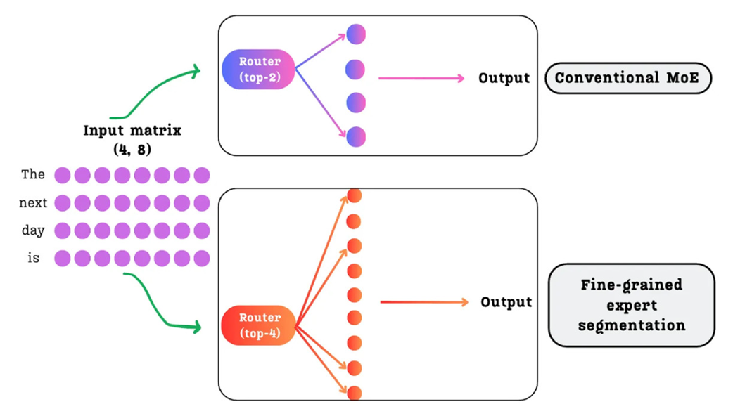
As illustrated in Figure 4.20, instead of one FFN being replaced by a few large experts, it is replaced by a much larger pool of smaller, more specialized experts.

How does this work without increasing the total model size or computational cost?

This is a critical point. The total number of learnable parameters and the computational cost during inference do not necessarily increase. This is achieved by proportionally reducing the size of each individual expert as their total number grows.

For example, imagine a traditional expert is a large Feed-Forward Network with a hidden dimension of 4096.

• In a Conventional MoE with 16 experts, the total “expert capacity” is 16 * 4096.
• In a Fine-Grained MoE, we could have 64 experts, but the hidden dimension of each expert might be reduced to 1024. The total capacity remains the same (64 * 1024 = 16 * 4096).

The total number of expert parameters and the number of activated parameters (top-k) can remain the same. We are not making the model bigger; we are just dividing its knowledge into a larger number of more specialized containers.

This architectural change directly solves the knowledge hybridity problem:

• With a vast number of experts available (e.g., 64 or 256 instead of 16), the model is no longer forced to cram diverse knowledge into a single expert.
• The routing mechanism now has a much wider and more specialized pool of experts to choose from. It can learn to bank tokens to highly specific experts. There can now be a dedicated expert just for Python syntax errors, another for legal terminology, and another for poetic metaphors.

By increasing the number of available specialists, each expert can become a true master of their narrow domain. This allows the model as a whole to achieve a much more nuanced and powerful understanding of language, which was a key factor in DeepSeek’s strong performance on a wide range of benchmarks.

4.4.3 Innovation #2: Shared expert isolation

Fine-grained segmentation is a powerful tool for increasing specialization, but it doesn’t solve the second core problem DeepSeek identified: Knowledge Redundancy.

This problem occurs because many different types of tokens require some common, foundational knowledge to be processed correctly. For example, an expert specializing in Python syntax and an expert specializing in legal contracts both need a fundamental understanding of English grammar. In a traditional MoE model, both of these experts would be forced to waste a portion of their parameter capacity learning and storing the same redundant grammatical knowledge. This hinders their ability to become even more specialized in their primary tasks.

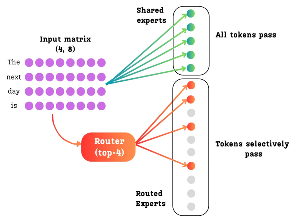
To solve this, DeepSeek introduced a brilliant architectural change: Shared Expert Isolation. They divided the experts in each MoE layer into two distinct and functionally different groups.

1. Routed Experts: These are the fine-grained, specialized experts we just discussed. They are activated sparsely. A token is only sent to the top-$k$ routed experts as determined by the router. These are the specialists.
2. Shared Experts: This is a small, separate set of experts that are dense. Every single token that enters the MoE layer is processed by all of the shared experts, regardless of the router’s decision. These are the generalists.

This clever division of labor is a direct solution to the knowledge redundancy problem:

• The Shared Experts, because they see every single token, naturally learn the common, foundational knowledge that is required across all domains (e.g., general grammar, common sense facts, basic reasoning structures). They become the central repository for this shared information, eliminating the need for it to be duplicated.
• The Routed Experts are now freed from this burden. They no longer need to waste their capacity re-learning redundant information. They can dedicate their entire parameter budget to becoming hyper-specialized in their unique, narrow domains.

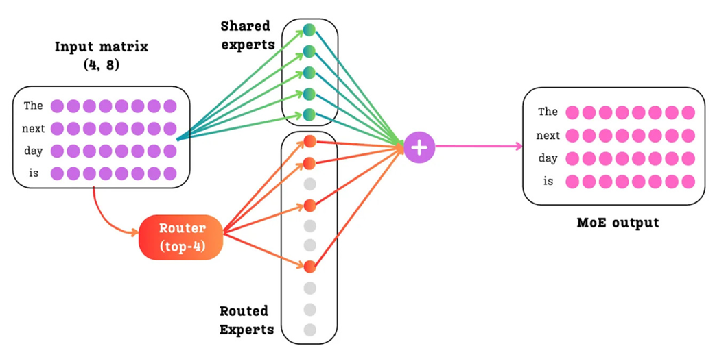
The final step is to combine the knowledge from both paths. The output of the MoE layer is the sum of the outputs from the dense shared experts and the weighted sum of the outputs from the selected routed experts.

Therefore, the final output for a given token $x$ is: \(\text{FinalOutput} = \text{Residual}(x) + \text{Sum}(\text{SharedOutputs}) + \text{Weighted\_Sum}(\text{RoutedOutputs})\)

By isolating the common knowledge into a shared, dense path, DeepSeek allows the sparse, routed experts to achieve a level of specialization that was previously not possible. This combination of fine-grained segmentation and shared experts is what enables the model to be both incredibly knowledgeable and highly efficient. However, there was one final piece of the puzzle they addressed in their V3 model: the load balancing mechanism itself.

4.4.4 Innovation #3: Auxiliary-loss-free load balancing

In section 4.3, we explored the traditional methods for ensuring that the workload is distributed evenly across experts, namely the Auxiliary Loss and the Load Balancing Loss. While these methods are effective, they come with a significant drawback: they interfere with the model’s main training objective.

Let’s quickly recap the problem. The total loss that the model tries to minimize becomes a combination of two different goals:

\[\text{TotalLoss} = \text{NextTokenPredictionLoss} + \lambda \cdot \text{BalancingLoss}\]

This creates a difficult trade-off:

• If the scaling factor $\lambda$ is too low, the balancing loss is ignored, and experts can become imbalanced, hurting performance.
• If $\lambda$ is too high, the model focuses too much on balancing the experts and not enough on its primary task of learning the language, which also hurts performance.

Finding the perfect balance is difficult and can compromise the final quality of the model. This is the problem DeepSeek set out to solve with their V3 architecture. They asked: Is it possible to enforce load balance without using an additional loss term at all?

The answer is yes, and the solution is a brilliant dynamic adjustment mechanism they call Auxiliary-Loss-Free Load Balancing.

The core idea: Dynamically adjusting router scores with a bias term

Instead of penalizing the model after the fact with a loss term, this new technique intervenes directly in the routing process before the experts are selected. It does this by adding a learnable bias term to the raw scores produced by the router.

The core logic is as follows:

1. At the end of each training step, we calculate the load for each expert.
2. We identify which experts were overloaded (received more tokens than average) and which were underloaded (received fewer).
3. We then adjust the bias term for the next training step:
   • For underloaded experts, we increase their bias.
   • For overloaded experts, we decrease their bias.

This creates a self-correcting dynamic system. By increasing the bias for an underloaded expert, we are artificially inflating its scores in the next step, making the router more likely to select it. Conversely, by decreasing the bias for an overloaded expert, we are making it less likely to be chosen.

Let’s walk through this step-by-step with our example.

A. Calculating the Expert Load and Load Violation

The first step in this dynamic process is to measure how balanced the routing was in the current training batch. We start with our Expert Selector Weight Matrix, which contains the final probabilities for each expert for each token.

First, we determine the total number of tokens routed to each expert. For simplicity in this calculation, a token is considered “routed” to any expert for which it has a non-zero probability.

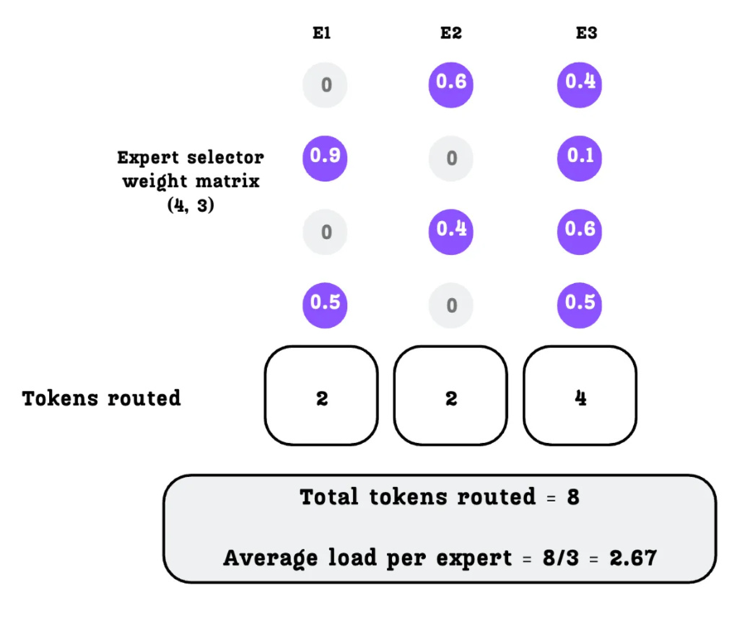
As shown in Figure 4.23:

• Expert 1 is selected for 2 tokens.
• Expert 2 is selected for 2 tokens.
• Expert 3 is selected for 4 tokens.

The total number of routed tokens across all experts is 2 + 2 + 4 = 8. With 3 experts, the average load per expert is 8 / 3 = 2.67 tokens.

Now we can determine which experts are overloaded or underloaded by calculating the load violation.

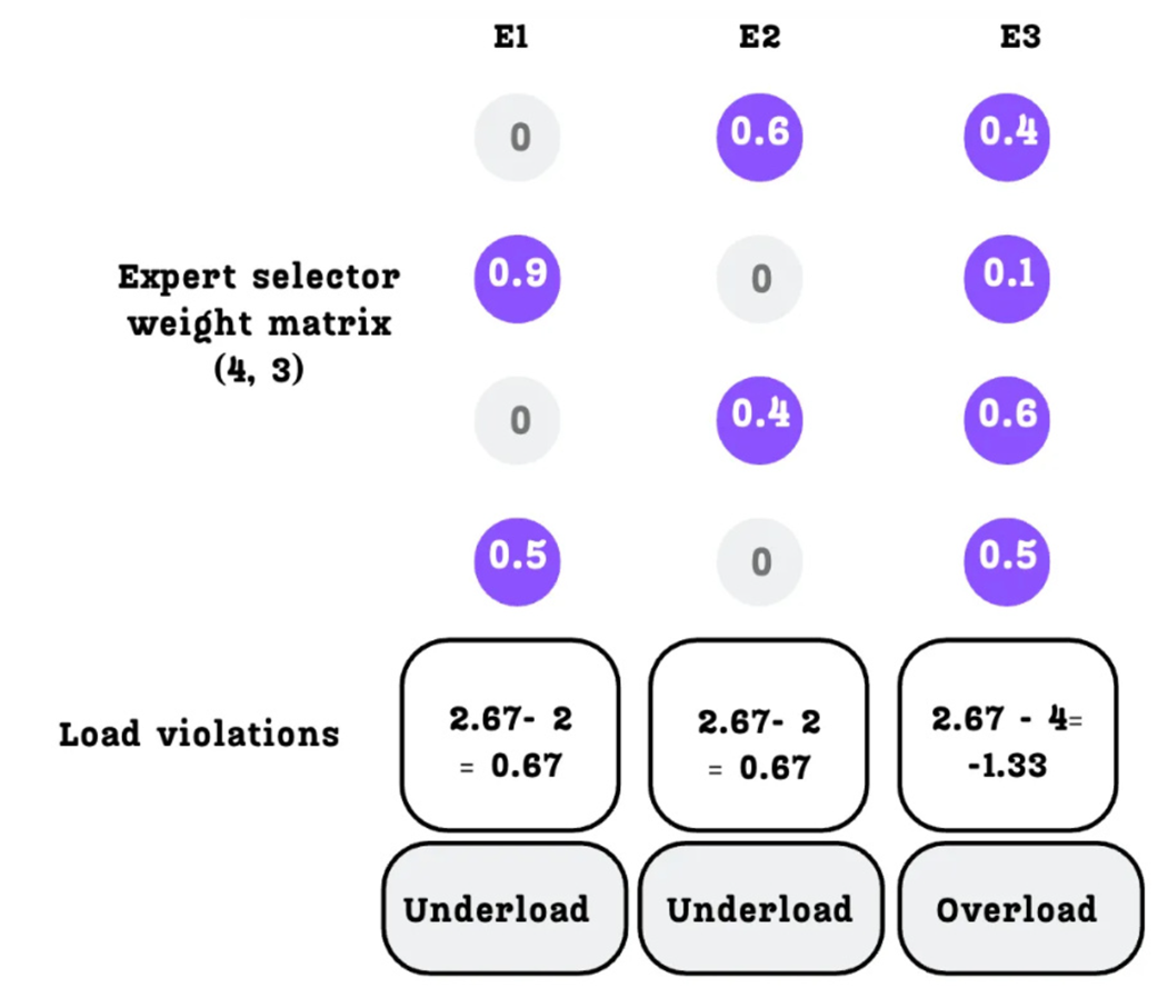
The load violation is simply the difference between the average load and the actual load:

• Expert 1: 2.67 - 2 = 0.67 (Positive violation = Underloaded)
• Expert 2: 2.67 - 2 = 0.67 (Positive violation = Underloaded)
• Expert 3: 2.67 - 4 = -1.33 (Negative violation = Overloaded)

We now have a clear signal for each expert: E1 and E2 need to be chosen more often, and E3 needs to be chosen less often.

B. Updating the Bias Term

Next, we use this load violation signal to update a persistent bias term ($b_i$) for each expert. Each expert has its own bias value, which is initialized to zero. At the end of each training step, we update it using the following simple formula:

\[b_i = b_i + \mu \cdot \text{sign}(\text{LoadViolation})\]

Here, $\mu$ is a small, predefined constant (like a learning rate) that controls the magnitude of the adjustment. The sign() function simply returns +1 if the error is positive (indicating the expert was underloaded) and -1 if it is negative (indicating the expert was overloaded).

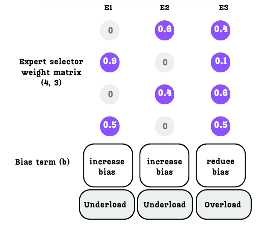
As shown in Figure 4.25, this simple rule means:

• For Expert 1 and 2 (underloaded, positive violation), we increase their bias.
• For Expert 3 (overloaded, negative violation), we reduce its bias.

This updated bias term is then carried over to the next training step.

C. Applying the Bias to the Router Logits

This is where the entire system comes together. In the next training step, when the router calculates its raw scores (the Expert Selector Matrix or logits), we add our newly updated bias term to these scores before the top-$k$ selection and softmax normalization.

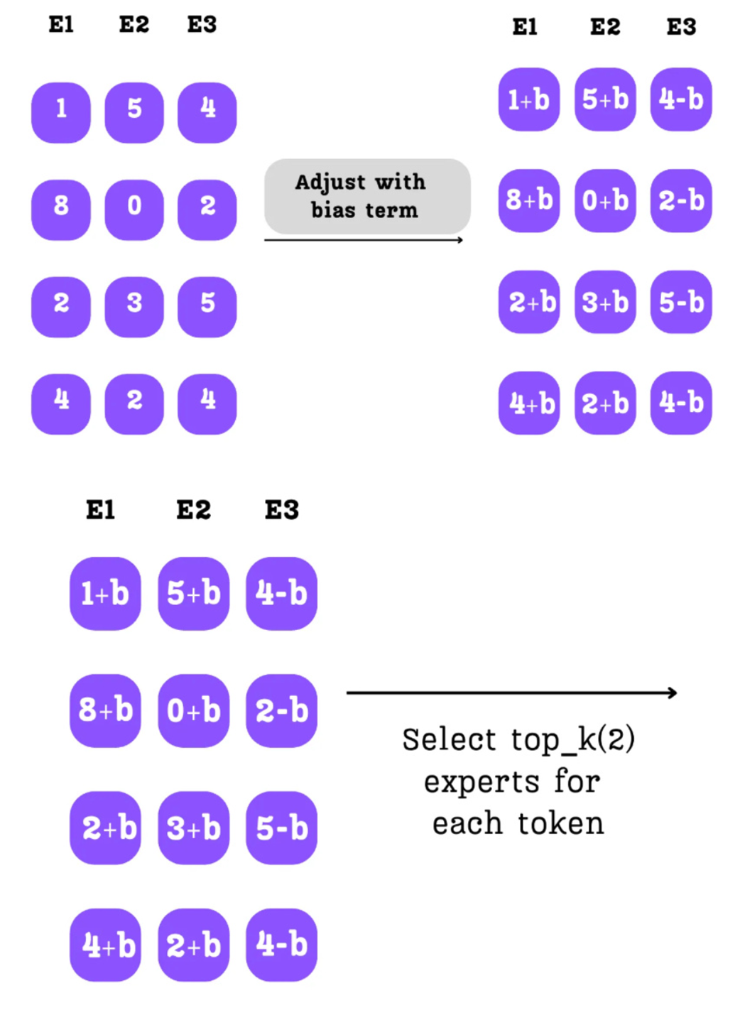
Let’s trace the effect as shown in Figure 4.26:

1. Original Logits: The router produces its initial scores.
2. Bias Adjustment: We add the bias $b$ we calculated from the previous step. a. The scores for Experts 1 and 2 (which were underloaded) are increased. b. The scores for Expert 3 (which was overloaded) are decreased.
3. New Top-K Selection: The top-k selection is now performed on these adjusted scores.

The effect is immediate. By increasing the scores for E1 and E2, we make it more likely that they will be among the top-2 experts selected by the router. By decreasing the score for E3, we make it less likely to be chosen.

This creates a dynamic, self-correcting feedback loop:

• If an expert is underutilized, its bias increases, making it more attractive to the router in the future.
• If an expert is overutilized, its bias decreases, making it less attractive to the router in the future.

Over the course of training, this system naturally pushes the router towards a state of equilibrium, ensuring all experts receive a relatively balanced load of tokens.

The Advantage of the Loss-Free Approach

This is an amazing innovation because it decouples the primary objective of learning language from the secondary task of load balancing. While traditional methods had a competing loss term, this dynamic bias adjustment allows the gradients that update the model’s core parameters (like the attention weights and the expert FFNs) to be derived purely from the next-token prediction loss. This separation allows the model to focus its gradient-based learning entirely on its primary task. The result is a more stable and efficient training process that improves both the model’s final performance and its overall load balance, solving the core trade-off of older MoE architectures.

This is what DeepSeek’s paper means when it says this method “achieves both better performance and better load balance.” By decoupling the two objectives, the model is free to focus 100% of its gradient-based learning on the primary task of understanding language, while this elegant bias mechanism handles the secondary task of keeping the experts balanced.

4.5 Building a complete DeepSeek-MoE language model from scratch

We have explored the core mechanics of Mixture-of-Experts, the challenge of load balancing, and the advanced solutions pioneered by DeepSeek. Now, we will integrate all these concepts into a single, functional PyTorch module. We will build the DeepSeekMoE class step-by-step, starting with its initialization. The complete code for this chapter is available in the book’s GitHub repository, and we encourage you to follow along: https://github.com/VizuaraAI/DeepSeek-From-Scratch/tree/main/ch04.

Let’s visualize the entire forward pass. Figure 4.27 provides a complete roadmap of the DeepSeekMoE module we are about to build, showing how it processes an input tensor $x$.

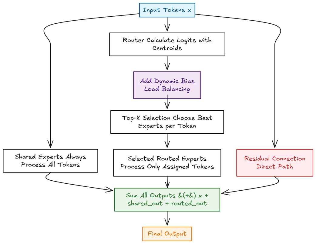
As the figure illustrates, our module’s logic is built around three parallel paths that are combined at the end:

1. The Shared Path: Every input token is processed by a small set of “generalist” shared experts. This dense path ensures that common, foundational knowledge is consistently applied.
2. The Routed Path: This sparse path is the core of the MoE mechanism. It involves a sequence of steps: calculating expert scores (logits), applying the dynamic bias for load balancing, selecting the top-$k$ experts, and finally processing tokens only through their assigned specialists.
3. The Residual Connection: A direct path for the original input $x$, which is crucial for stable training and preserving information from the previous layer.

These three outputs are then summed together—$x + \text{shared_out} + \text{routed_out}$—to produce the final result. With this blueprint in mind, let’s begin by defining the smallest building block of our system.

Step 1: Defining the Expert FFN

In the DeepSeek architecture, this is a two-layer MLP that performs the same “expansion-contraction” sequence we saw in dense models, though typically with a smaller hidden dimension. The code below defines this ExpertFFN, which includes a GELU activation function.

Listing 4.1 The ExpertFFN Module

import torch
import torch.nn as nn
import torch.nn.functional as F
import math
from typing import Optional

def _gelu(x: torch.Tensor) -> torch.Tensor:
    # Slightly faster GELU (approx)
    return 0.5 * x * (1.0 + torch.tanh(math.sqrt(2.0 / math.pi) *
    (x + 0.044715 * torch.pow(x, 3))))
 
class ExpertFFN(nn.Module):
    """
    A 2-layer MLP expert. Hidden dim is usually smaller than a dense FFN
    (e.g., 0.25 × d_model in DeepSeek-V3).
    """
    def __init__(self, d_model: int, hidden: int, dropout: float = 0.0):
        super().__init__()
        self.fc1 = nn.Linear(d_model, hidden, bias=False)
        self.fc2 = nn.Linear(hidden, d_model, bias=False)
        self.dropout = nn.Dropout(dropout)
 
    def forward(self, x: torch.Tensor) -> torch.Tensor:
        return self.fc2(self.dropout(_gelu(self.fc1(x))))

At its heart, each “expert” in an MoE layer is simply a standard Feed-Forward Network (FFN). In the DeepSeek architecture, this is a two-layer MLP that performs the same “expansion-contraction” sequence we saw in dense models, though typically with a smaller hidden dimension. The code above defines this ExpertFFN, which includes a GELU activation function.

Step 2: Initializing the MoE Layer

The __init__ method sets up all the components of our MoE layer. This includes creating the ModuleLists for our two distinct groups of experts: a small set of shared experts that every token will see, and a much larger pool of routed experts that will be used sparsely.

Crucially, it also sets up the parameters for the routing mechanism. This includes the centroids (the learnable weight matrix for the router) and the bias, a non-trainable buffer that will be dynamically updated to enforce load balancing without an auxiliary loss.

Listing 4.2 The DeepSeekMoE __init__ Method

class DeepSeekMoE(nn.Module):
    def __init__(
        self,
        d_model: int,
        n_routed_exp: int,
        n_shared_exp: int = 1,
        top_k: int = 8,
        routed_hidden: int = 2_048,
        shared_hidden: Optional[int] = None,
        bias_lr: float = 0.01,
        fp16_router: bool = False,
    ):
        super().__init__()
        assert top_k <= n_routed_exp, "k must be <= number of routed experts"
 
        self.d_model = d_model
        self.n_routed = n_routed_exp
        self.n_shared = n_shared_exp
        self.top_k = top_k
        self.bias_lr = bias_lr
        self.fp16_router = fp16_router
 
        # A) Creates the large pool of specialized, sparsely-activated experts.
        self.routed = nn.ModuleList(
            [ExpertFFN(d_model, routed_hidden) for _ in range(n_routed_exp)]
        )
 
        # B) Creates the small set of generalist experts, activated for every token.
        hidden_shared = shared_hidden or routed_hidden
        self.shared = nn.ModuleList(
            [ExpertFFN(d_model, hidden_shared) for _ in range(n_shared_exp)]
        )
 
        # C) The learnable experts centroid (router). 
        # The router calculates expert routes by measuring the similarity (dot product) 
        # between each token’s representation and each expert’s centroid vector.
        self.register_parameter("centroids",
            nn.Parameter(torch.empty(n_routed_exp, d_model)))
        nn.init.normal_(self.centroids, std=d_model ** -0.5)
 
        # D) The non-trainable bias for auxiliary-loss-free load balancing.
        self.register_buffer("bias", torch.zeros(n_routed_exp))

Step 3: The Forward Pass - The Shared Expert Path

The forward method begins by processing the input $x$ through the shared experts. As we discussed in the theory, this is a dense operation: every token in the batch is passed through every expert in the self.shared list.

This path ensures that common, foundational knowledge (like grammar or basic facts) is handled by a consistent set of parameters, solving the “knowledge redundancy” problem. The output from these experts forms a base result, which will then be refined by the specialized routed experts.

Listing 4.3 The Shared Expert Path in the forward Method

    def forward(self, x: torch.Tensor) -> torch.Tensor:
        B, S, D = x.shape
        x_flat = x.reshape(-1, D)  # [N, D] with N=B*S
 
        # 1) shared path
        shared_out = torch.zeros_like(x_flat)
        for exp in self.shared:
            shared_out += exp(x_flat)
 
        # ... (routed path comes next)

In this section of the code, we first reshape the input tensor for easier processing. We then initialize an output tensor shared_out and iterate through our list of shared experts, accumulating their results. Note that for simplicity and clarity, our implementation processes the shared experts sequentially in a for loop. In a production-level framework, these expert computations would be performed in parallel to maximize throughput. Every token is processed by every shared expert, creating a dense output that captures the generalist knowledge required for the entire batch.

Step 4: The Forward Pass - The Routed Expert Path

This is where the sparse part of the MoE architecture comes into play. After the shared experts have processed the tokens, the routing mechanism takes over to select a small, specialized subset of “routed” experts for each token. This section of the forward pass handles the entire routing and dispatching logic.

The process involves four key stages:

1. Calculate Router Logits: A linear layer (the “router”) calculates a raw score for each expert for every token.
2. Apply Dynamic Bias: The auxiliary-loss-free bias term is added to these scores to dynamically encourage a balanced load.
3. Top-K Gating: A topk operation selects the best experts, and a softmax function converts their scores into normalized weights.
4. Dispatch and Combine: Each token is sent to its chosen experts, and their outputs are combined in a weighted sum.

Listing 4.4 The Routed Expert Path and Final Combination

        # ... (shared path from previous listing)
 
        # 2) router logits in (optional) mixed precision
        # A) The router calculates raw scores for each expert.
        use_autocast = self.fp16_router and x.is_cuda
        device_type = "cuda" if x.is_cuda else x.device.type
        with torch.autocast(device_type=device_type, enabled=use_autocast):
            logits = F.linear(x_flat, self.centroids)
            
            # B) The dynamic bias is added to the scores to enforce load balancing.
            logits = logits + self.bias.to(logits.dtype)
 
        # C) Sparsity in action: top-k selects the experts and softmax computes their weights.
        topk_logits, topk_idx = torch.topk(logits, self.top_k, dim=-1)
        gate = F.softmax(topk_logits, dim=-1, dtype=x.dtype)
 
        # 3) dispatch per expert (correct indexing)
        routed_out = torch.zeros_like(x_flat)
        for i in range(self.n_routed):
            # D) Efficiently identifies all tokens that should be routed to the current expert `i`.
            mask = (topk_idx == i)
            row_idx, which_k = mask.nonzero(as_tuple=True)
            if row_idx.numel() == 0:
                continue
            
            exp_in = x_flat.index_select(0, row_idx)
            out = self.routed[i](exp_in)
            w = gate[row_idx, which_k].unsqueeze(-1)
            
            # E) The weighted outputs from the expert are added back to their original token positions.
            routed_out.index_add_(0, row_idx, out * w)
 
        routed_out = routed_out.view(B, S, D)
        
        # F) The final output is the sum of the residual, shared, and routed paths.
        return x + shared_out.view(B, S, D) + routed_out

The logic here is a highly effective implementation of sparse dispatch. Instead of sending tokens one by one, we process all tokens destined for a single expert in a batch. The loop iterates through each expert i. Inside the loop, (topk_idx == i) creates a boolean mask to identify which tokens have selected expert i. The nonzero() function gives us the indices of these tokens (row_idx). We then select these tokens, pass them through the expert, weight their outputs using the gate values, and use index_add_ to add the results back to the correct positions in the routed_out tensor.

Finally, the original input x, the output from the shared experts shared_out, and the output from the routed experts routed_out are summed together to produce the final output of the MoE layer.

Step 5: The Auxiliary-Loss-Free Bias Update

We have now implemented a complete DeepSeekMoE forward pass. The final component is the dynamic adjustment mechanism that ensures our experts remain balanced over time. This is handled by the update_bias method, which is called once per training step.

This function operates @torch.no_grad(), meaning its operations do not contribute to the model’s gradients. Its sole purpose is to calculate the current expert load, determine which experts are over- or under-utilized, and apply a small adjustment to the self.bias buffer. This adjustment will then influence the routing decisions in the next forward pass, creating the self-correcting feedback loop we discussed in the theory.

Listing 4.5 The update_bias Method for Load Balancing

    @torch.no_grad()
    def update_bias(self, x: torch.Tensor):
        # Call once per optimizer step on the same tokens seen by forward.
        # Uses the SAME logits (including current bias) to estimate loads.
        
        N = x.shape[0] * x.shape[1]
        
        # A) Recalculates the logits using the current bias to accurately measure the load.
        logits = F.linear(x.reshape(-1,
            self.d_model), self.centroids) + self.bias
        
        _, idx = torch.topk(logits, self.top_k, dim=-1)
 
        # B) Efficiently counts how many tokens were routed to each expert using bincount.
        counts = torch.bincount(idx.flatten(),
            minlength=self.n_routed).float()
        
        avg = counts.sum() / max(1, self.n_routed)
 
        # Smooth, bounded update; avoids large jumps from sign()
        # C) Calculates the load violation; a positive value indicates an under-loaded expert.
        violation = (avg - counts) / (avg + 1e-6)
 
        # D) Updates the bias term to influence the next training step's routing decisions.
        self.bias.add_(self.bias_lr * torch.tanh(violation))

The logic is a direct implementation of the theory:

1. It recalculates the router logits for the batch, including the current bias.
2. It performs a topk selection to find the chosen experts for each token.
3. torch.bincount efficiently counts how many tokens were routed to each expert.
4. It calculates the “load violation” for each expert—a positive value for under-loaded experts and a negative one for over-loaded experts.
5. Finally, it updates self.bias by adding a small, scaled value of this violation. The torch.tanh function is used to smooth the update and prevent extreme jumps, ensuring a stable adjustment process.

This concludes our from-scratch implementation of the DeepSeekMoE layer. By breaking the code into these four distinct parts, we have seen how each theoretical concept—shared experts, sparse routing, and dynamic balancing—is translated into a functional and efficient PyTorch module.

4.6 The payoff: An empirical head-to-head comparison

Having explored the theoretical underpinnings of both the traditional Mixture-of-Experts architecture and the advanced solutions pioneered by DeepSeek, it’s time to put our knowledge to the test. Theory is one thing, but empirical results provide the final verdict. To that end, we conducted a head-to-head comparison by building and training two models from scratch: a baseline “Standard MoE” using a conventional load balancing loss, and our innovative “DeepSeek-MoE” implementing shared experts and auxiliary-loss-free dynamic balancing.

Our goal is to answer a simple question: Do these architectural innovations actually lead to a better and more efficient model? The complete code used to run this experiment and generate the following results is available for you to explore and replicate in the book’s GitHub repository.

Bonus Code Link: https://github.com/VizuaraAI/DeepSeek-From-Scratch/tree/main/ch04/02-bonus-code

Let’s begin our analysis by looking at the most important metric: the validation loss. This tells us how well each model is generalizing to new, unseen data throughout the training process. The plot in Figure 4.28 tracks the validation loss for both models over 5,000 training iterations.

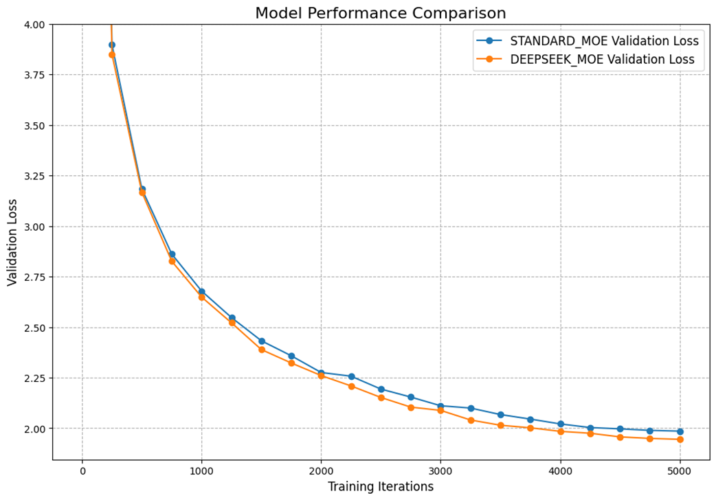
As the learning curves illustrate, both models successfully learn to process the TinyStories dataset. However, a clear trend emerges. From the very early stages of training, the DeepSeek-MoE model consistently achieves a lower validation loss than its standard counterpart. While the difference isn’t dramatic, a result of the relatively small model size and the less diverse nature of the training data, the advantage is consistent and widens slightly over time. This is our first piece of evidence that the DeepSeek architecture enables more effective learning.

While the loss curve gives us a great overview of learning performance, a detailed metrics table allows us to quantify the “total payoff” by looking at performance and computational efficiency side-by-side. Table 4.1 provides a comprehensive summary of the training run for both models, which were configured to have a nearly identical number of learnable parameters for a fair comparison.

Table 4.1 Comparison of training run

Model	Parameters (M)	Training Time (min)	Throughput (iter/min)	Best Val Loss
STANDARD_MOE	101.30	14.29	350.0	1.9854
DEEPSEEK_MOE	101.28	11.67	428.6	1.9451

Not only did the DeepSeek-MoE model achieve a lower final validation loss (1.9451 vs. 1.9854), but it was also significantly faster. It completed the training run in just 11.67 minutes, demonstrating a throughput of 428.6 iterations per minute, a 22% increase over the standard MoE’s 350.0 iter/min. This proves that the DeepSeek architecture is not just more effective at learning, but it is also more computationally efficient.

The key difference between the two models lies in their approach to load balancing. The standard MoE uses an auxiliary loss to encourage balance over the entire training run, while the DeepSeek-MoE uses a dynamic bias to enforce it on a more immediate, per-batch basis.

Figure 4.29 visualizes the inherent challenge that the standard MoE faces. The bar chart shows how many tokens from a single validation batch were routed to each of the 22 experts in its first layer.

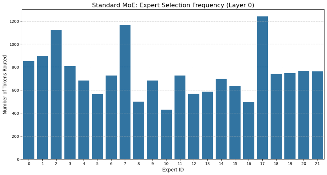
The chart clearly shows a significant load imbalance. Some experts, like #7 and #17, have become “hotspots,” processing a disproportionately high number of tokens. Conversely, others, like #10 and #16, are underutilized. While the auxiliary loss aims to even this out over thousands of iterations, it struggles to prevent these imbalances from occurring within individual batches. This inefficiency means that some experts become computational bottlenecks while the knowledge capacity of others is wasted.

Now, Figure 4.30 shows the expert utilization for the same validation batch, but this time processed by our DeepSeek model.

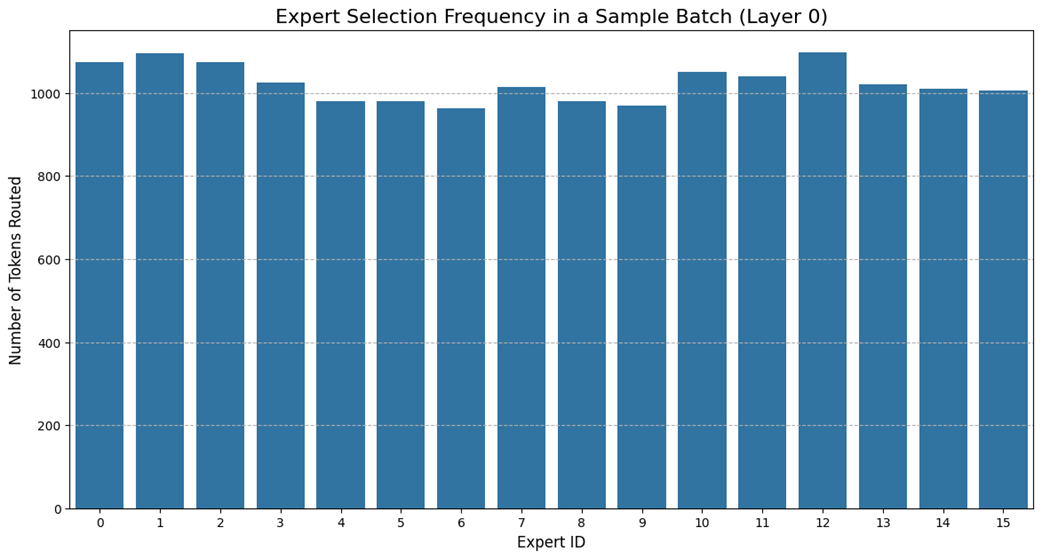
The auxiliary-loss-free dynamic bias mechanism has done its job perfectly, resulting in a remarkably uniform load distribution. The self-correcting system, which penalizes overloaded experts and rewards underloaded ones in real-time, ensures that the workload is spread evenly across all available specialists. This is the tangible proof of the architecture’s efficiency: no single expert becomes a bottleneck, and the full parallel processing power of the committee is leveraged effectively.

Our head-to-head experiment provides a clear verdict. The architectural innovations of the DeepSeek-MoE model, specifically its combination of powerful shared generalists and the elegant auxiliary-loss-free mechanism for balancing its specialists, are not merely theoretical. They deliver tangible benefits in both performance and efficiency. By decoupling the task of load balancing from the primary learning objective, the model learns better and faster. This is the core principle that allows DeepSeek to scale intelligence so efficiently, providing a powerful blueprint for the future of large-scale language models.

In the next chapter, we will dive into further performance and memory optimizations, exploring advanced techniques like Multi-Head Latent Attention (MLA) and FP8 quantization that push the boundaries of large language model efficiency.

4.7 Summary

• Dense Feed-Forward Networks (FFNs) in standard Transformers are computationally expensive, as all of their parameters are activated for every single token, creating a bottleneck for both training and inference.
• Mixture of Experts (MoE) replaces the single, dense FFN with a committee of smaller, specialized “expert” networks.
• The efficiency of MoE comes from sparsity: for any given token, a routing mechanism activates only a small subset of the total experts (e.g., the top 2), leaving the rest dormant and their computations unperformed.
• During pre-training, experts learn to specialize in handling specific types of information (e.g., punctuation, verbs, or Python code), which is why activating only a few is effective.
• The routing mechanism is a small, learnable linear layer that generates scores for each expert. A top-k selection identifies the most relevant experts, and a softmax function converts their scores into weights for combining their outputs.
• Imbalanced routing, where some experts are over-utilized and others are ignored, leads to inefficient learning and performance degradation.
• Traditional MoE models use an Auxiliary Loss term to penalize imbalance, but this can interfere with the primary training objective of learning the language.
• DeepSeek’s first innovation, Fine-Grained Expert Segmentation, uses a massive number of smaller experts to solve the problem of Knowledge Hybridity, allowing for deeper specialization.
• DeepSeek’s second innovation, Shared Expert Isolation, uses a small set of dense “generalist” experts to learn common knowledge, solving the problem of Knowledge Redundancy and freeing up the routed “specialist” experts.
• DeepSeek’s third innovation, Auxiliary-Loss-Free Load Balancing, dynamically adjusts router scores with a bias term, enforcing balance without interfering with the main training loss and resolving the core trade-off of traditional balancing methods.