5 Multi-token prediction and FP8 quantization
This chapter covers
- Multi-Token Prediction for stronger training signals
- Implementing a causal MTP architecture
- Utilizing FP8 quantization to optimize training efficiency
We have now established the core architectural pillars of the DeepSeek model: Multi-Head Latent Attention and Mixture-of-Experts. These innovations define what the model computes. Now, we turn our attention to an equally important topic that defines how these computations are performed with incredible efficiency. This involves two key techniques that are central to DeepSeek’s training methodology: Multi-Token Prediction (MTP) and FP8 Quantization. While FP8 quantization was already being adopted in the industry to accelerate inference, DeepSeek’s key innovation was demonstrating its successful and stable application to the much more demanding task of large-scale training.
This chapter is divided into two main parts. First, we will dive deep into MTP, understanding its motivation, advantages, and exactly how DeepSeek implemented their advanced, causal version of it. You will learn not just the theory but also how to build a functional MTP module, seeing firsthand how predicting a horizon of tokens strengthens the model’s planning capabilities. After mastering MTP, we will move to the second part, a deep dive into the FP8 Quantization framework that allows these massive models to be trained with remarkable speed and memory efficiency.
Now let’s look at the roadmap for these mechanisms. As illustrated in figure 5.1, our roadmap highlights the components we will build in this chapter.
Figure 5.1 Our four-stage journey to build the DeepSeek model. This chapter focuses on the highlighted components, Multi-Token Prediction (MTP) and FP8, which are the major innovations in the advanced training pipeline.
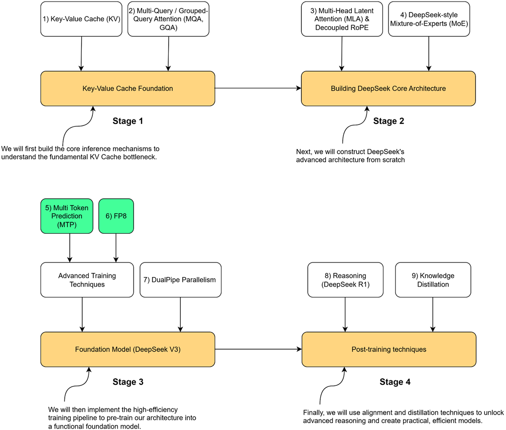
This chapter concludes Stage 3 of our journey. By implementing these high-efficiency training techniques, you will gain a practical understanding of how modern LLMs are trained at scale. This knowledge is not just theoretical; it provides the final set of tools needed to pre-train a functional foundation model, setting the stage for the alignment and distillation techniques we will cover in the final part of the book.
Let’s begin by exploring the powerful idea of predicting more than one token at a time.
5.1 The core idea: From single-token to multi-token prediction
The entire training process for the language models we’ve discussed so far has been based on a single, simple objective: Next-Token Prediction. In the standard approach, we give the model a sequence of input tokens. These tokens are processed through a series of Transformer blocks (the “Shared Transformer Trunk”), and for each input token, the model’s goal is to predict the single token that immediately follows it.
Figure 5.2 The standard single-token prediction process. For a given sequence of input tokens, the model predicts only the single immediate next token for each position.
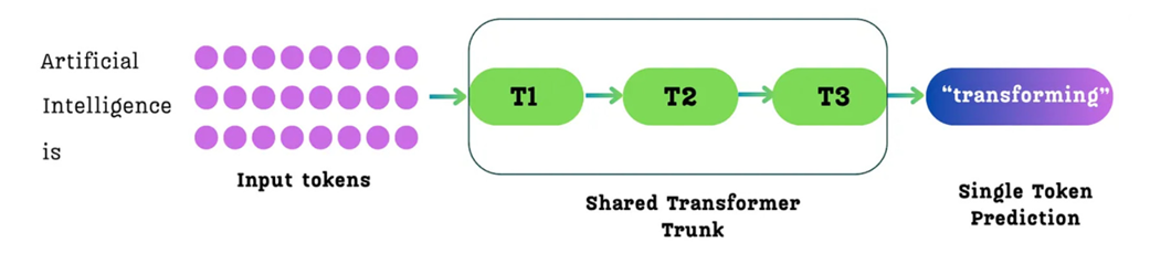
As shown in figure 5.2, for an input like “Artificial Intelligence is,” the model processes these three tokens. For the token “is,” its primary training goal is to predict the single next token, “transforming.” While it also makes predictions for the other tokens (e.g., predicting “Intelligence” after “Artificial”), the learning signal at each position is focused on a horizon of just one step into the future.
Multi-Token Prediction, as the name suggests, changes this fundamental objective. Instead of predicting only the single next token, the model is trained to predict multiple future tokens at once.
Figure 5.3 The Multi-Token Prediction (MTP) process. For a given sequence of input tokens, the model is trained to predict multiple future tokens simultaneously from each position. For example, from the input token “is,” it might predict the sequence “transforming,” “the,” “world.”
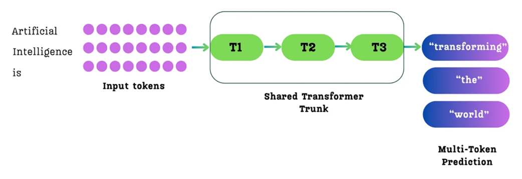
As illustrated in figure 5.3, when the model processes the input “Artificial Intelligence is,” it makes predictions from each token. In the standard single-token approach (figure 5.2), the primary goal for the token “is” would be to predict only the next token, “transforming.”
With MTP, the task is expanded. From the position of the token “is,” the model is now tasked with predicting a whole sequence of future tokens: “transforming,” “the,” and “world.” The loss is then calculated based on how well it predicted this entire future sequence from that position.
This seemingly simple change from predicting one token to predicting many has profound implications for the model’s training process and its final capabilities. It was not invented by DeepSeek but was explored in a paper from Meta AI researchers titled “Better and faster large language models via multi-token prediction.” (https://arxiv.org/pdf/2404.19737) DeepSeek took this powerful idea and integrated it with their own unique architectural innovations.
5.2 The four key advantages of MTP
Changing the training objective from predicting one token to predicting many is more than just a minor tweak; it fundamentally alters what the model learns and how efficiently it learns it. Four major benefits arise from this architectural shift, as demonstrated in the original MTP paper and leveraged by DeepSeek.
5.2.1 Densification of training signals
The first and most important advantage is that MTP provides much richer and denser training signals than single-token prediction. In traditional training, for each token, the model receives a gradient signal based on its ability to predict just one step ahead. It learns about immediate, local dependencies very well (e.g., that “Intelligence” is likely to follow “Artificial”).
With MTP, the learning signal is far more comprehensive. When the model processes the token “Artificial,” it’s not just getting feedback on its prediction of “Intelligence.” It’s also getting feedback on its ability to foresee “is,” “transforming,” “the,” and “world.”
This means that from a single training example, the model is forced to learn about longer-range structure, grammar, and coherence. It sees and learns the relationships across multiple future steps simultaneously. This richer gradient information guides the model’s internal representations towards better planning and forecasting of sequences. The training process becomes more efficient because every single training sample now contains much more information for the model to learn from.
5.2.2 Improved data efficiency
This densification of training signals leads directly to the second benefit: improved data efficiency. Since each training sample is now more informative, the model can achieve a higher level of performance with the same amount of training data.
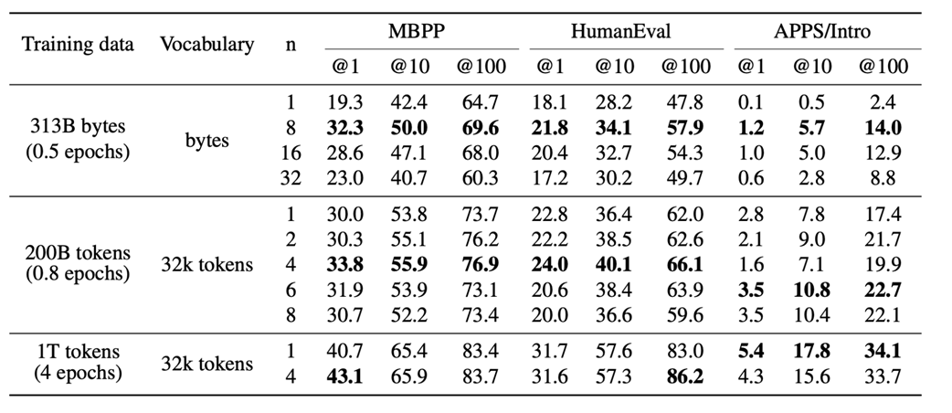
This isn’t just a theoretical benefit; it has been proven quantitatively. The original MTP paper demonstrated this on standard coding benchmarks like MBPP (Mostly Basic Python Problems) and HumanEval, as shown in figure 5.4.
Figure 5.4 Performance improvement of MTP over single-token prediction on coding benchmarks. Positive bars indicate MTP is better. (Source: Gloeckle et al., 2024)
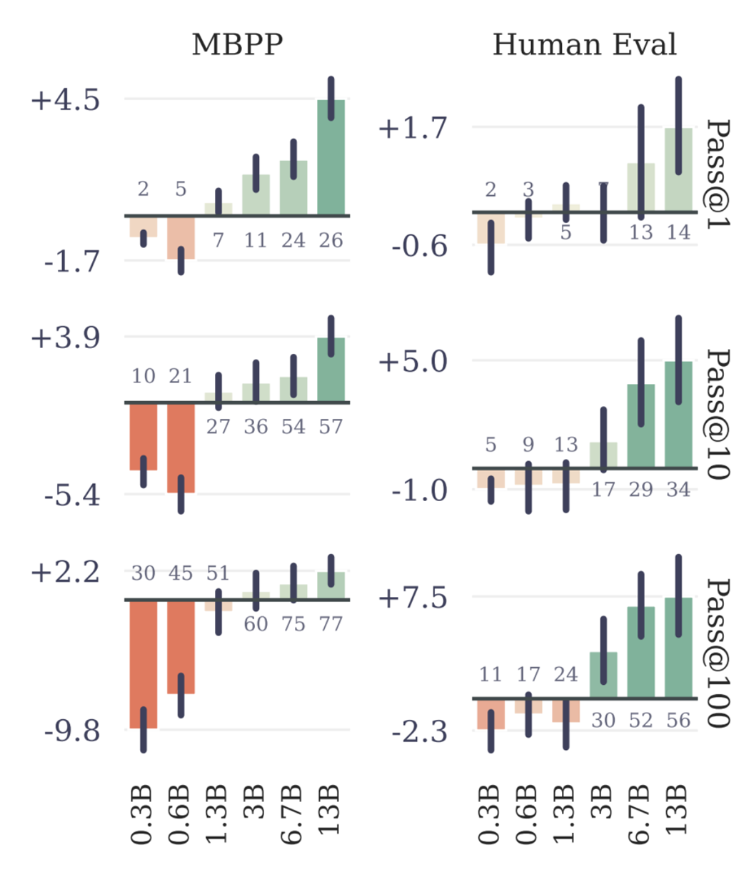
The data clearly shows that as models scale (from 0.3B to 13B parameters), the performance advantage of MTP becomes more pronounced and consistent. This establishes that MTP is a powerful technique for improving data efficiency. However, this raises a new question: if predicting multiple tokens is good, how many should we predict? The same study explored this by varying the number of predicted future tokens, denoted by n.
Figure 5.5 The effect of increasing the number of predicted future tokens (n) on benchmark performance. (Source: Gloeckle et al., 2024)
These results show two clear trends:
- As shown in figure 5.4, while MTP can sometimes perform worse on very small models, as the model size increases, it consistently and significantly outperforms the single-token baseline.
- As shown in figure 5.5, for a fixed amount of training data, increasing the number of predicted future tokens (n) generally leads to better performance on these benchmarks, up to a certain point.
This provides strong evidence that MTP allows the model to learn more effectively from the same data, a crucial advantage when training on massive, expensive datasets.
5.2.3 Better planning by prioritizing “choice points”
The third advantage of MTP is more subtle but incredibly powerful: it implicitly teaches the model to be better at planning by forcing it to pay more attention to the most important tokens in a sequence.
To understand this, we need to introduce the concept of a “choice point.” A choice point is a key token in a sequence that significantly influences the future outcome. Most transitions are simple and predictable (e.g., 1 -> 2, 2 -> 3), but some transitions represent a major shift in context (e.g., transitioning from numbers to letters).
Figure 5.6 MTP implicitly assigns higher weights to consequential “choice point” tokens. (Source: Gloeckle et al., 2024)
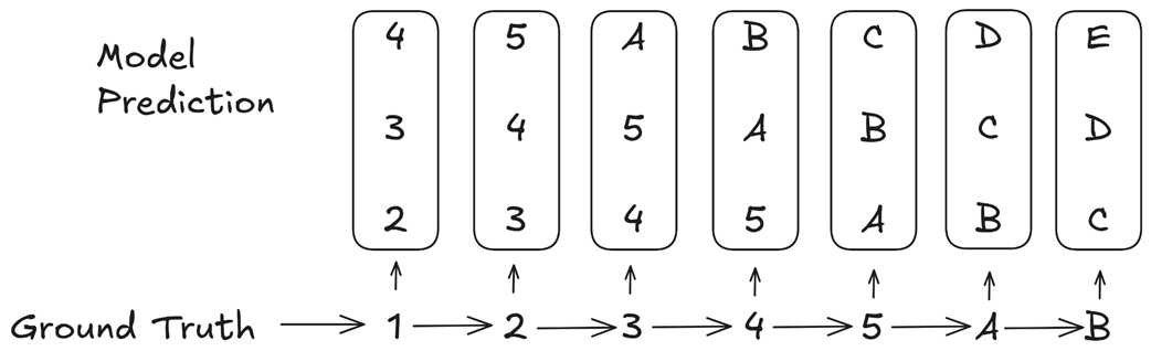
Let’s analyze the example in figure 5.6. The ground truth sequence is 1 -> 2 -> 3 -> 4 -> 5 -> A -> B. The transition from 5 -> A is the critical “choice point” where the pattern changes from numbers to letters.
Now, consider how the MTP loss is calculated. When the model sees the input token 3, it is trained to predict the next three tokens: 4, 5, A. The error associated with predicting A is part of the loss calculation for the input 3.
When the model sees the input 4, it is trained to predict 5, A, B. The error for A is part of the loss again. When it sees 5, it is trained to predict A, B, C, and the error for A is part of the loss a third time.
The errors related to predicting the consequential token A appear repeatedly in the overall loss calculation, far more often than the errors for the simple, inconsequential transitions. This means the multi-token prediction loss implicitly assigns a higher weight to these critical choice points.
The training process, therefore, naturally prioritizes getting these crucial, pattern-shifting tokens correct. This forces the model to develop better internal representations for planning and forecasting sequences, as it learns to recognize and correctly handle the most important decision points in the text.
5.2.4 Higher inference speed via speculative decoding
The fourth and final advantage is that MTP can lead to significantly faster inference, with observed speedups of up to 3x on certain tasks. This is achieved through a technique called speculative decoding. In standard autoregressive generation, we run the full, large language model once for every single token. This is slow.
Speculative decoding works differently:
- Drafting: A small, fast “draft” model (or an MTP head) generates a chunk of several candidate tokens at once.
- Verification: The main, large language model then processes this entire chunk in a single forward pass to verify which of the drafted tokens are correct.
Because a single forward pass over a chunk of tokens is much faster than multiple, sequential forward passes, this can dramatically speed up generation. MTP is a natural fit for this process, as the MTP heads can serve as the “draft” model, predicting multiple future tokens that the main model can then verify.
It’s important to note, as mentioned in the DeepSeek V3 paper, that they used MTP’s benefits primarily during pre-training to get the advantages of denser signals and better planning. For their public release, the inference was done using standard single-token prediction, discarding the MTP modules. However, they explicitly state that the MTP modules can be repurposed for speculative decoding to accelerate inference, highlighting the dual benefit of this powerful technique.
5.3 The DeepSeek MTP architecture: A visual and mathematical walkthrough
While the original MTP paper from Meta proved the concept’s effectiveness, it did so by predicting multiple future tokens using independent output heads. This means the prediction for the second future token was made without any information from the prediction for the first.
DeepSeek recognized a key opportunity for improvement. Their implementation is designed to sequentially predict additional tokens and keep the complete causal chain at each prediction depth. This means the prediction for future token t + 2 is informed by the prediction for token t + 1, creating a more coherent and powerful forecasting mechanism. Let’s break down their architecture step-by-step, starting with the initial input to the entire MTP process.
5.3.1 The starting point: The shared transformer trunk
The Multi-Token Prediction process does not start from the raw input tokens. Instead, it begins after the main body of the Transformer has already processed the input sequence.
An input sequence (e.g., “Artificial Intelligence is”) is first passed through what the original MTP paper calls the “Shared Transformer Trunk.” This is simply the standard stack of Transformer blocks that we are already familiar with (e.g., 61 blocks in DeepSeek-V3).
Figure 5.7 The initial step of the Multi-Token Prediction process. Input tokens are passed through the main “Shared Transformer Trunk,” which consists of multiple Transformer blocks. The output is the initial matrix of hidden states (denoted as h⁰ or z), which serves as the starting point for the MTP modules.
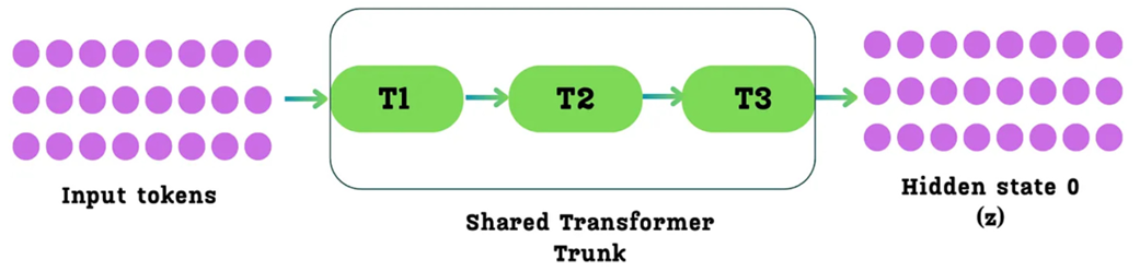
As shown in figure 5.7, the output of this main trunk is a matrix of hidden states. Let’s define this term precisely:
What is a Hidden State?
A hidden state is another name for the context vector that is output by a Transformer block. It is a rich, contextualized representation of an input token after it has been processed and has gathered information from its neighbors via the attention mechanism.
The output of the final Transformer block in the shared trunk is a matrix of these hidden states, one for each input token. For the purposes of MTP, we will call this initial matrix Hidden State 0, or h⁰, following the notation in the DeepSeek paper.
This h⁰ matrix is the starting point for the entire MTP process. It can be thought of as a stack of hidden state vectors, one for each token in the input sequence. For each token, its corresponding h⁰ vector will be fed into a chain of MTP modules to predict its future.
5.3.2 The MTP modules: A sequential chain of prediction
Instead of a single output head that predicts one token, the DeepSeek architecture uses a series of MTP Modules, one for each future token we want to predict. If we want to predict 3 future tokens (a prediction depth of D=3), we will have 3 MTP modules chained together.
The key innovation here is not just that these modules are dependent, but how that dependency is structured. Unlike approaches with independent prediction heads, DeepSeek’s modules form a causal chain. The refined hidden state from one module becomes the input for the next, allowing the model to sequentially refine its predictions at each future step. This architecture of cascaded latent refinement is what makes the forecasting mechanism so powerful and coherent.
Figure 5.8 The sequential architecture of the DeepSeek MTP modules. The hidden state from one module is passed as an input to the next, forming a causal chain.
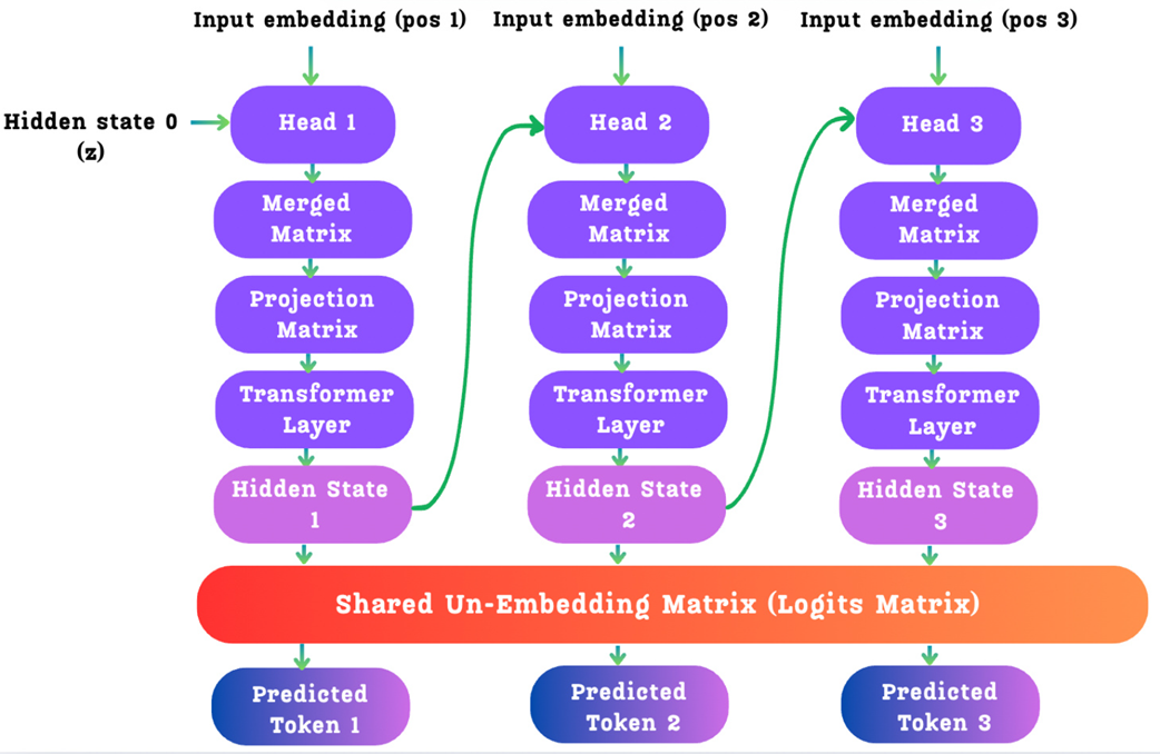
This diagram is the key to understanding DeepSeek’s innovation. Let’s trace the journey of a single input token’s h⁰ vector as it enters this chain. We will focus on the operations inside a single MTP module, for example, the first one, which we’ll call Head 1 (or k=1 for the prediction depth).
Each MTP head is a sophisticated piece of machinery designed to perform two jobs:
- Predict one future token.
- Generate a new, refined hidden state to pass to the next head in the chain.
Let’s look inside a single head to see how it achieves this.
Figure 5.9 The internal operations of a single MTP head.
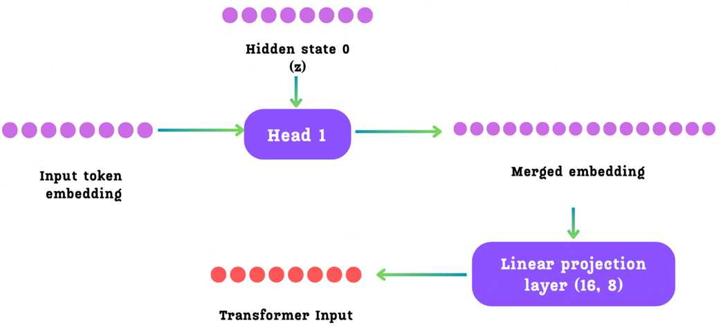
The operations within each head (k) can be broken down into the following steps:
Step 1: Gathering Inputs
Each head k takes two distinct inputs:
- The Hidden State (hᵏ⁻¹) from the previous head. For Head 1, this is the initial h⁰ from the main Transformer trunk.
- The Input Embedding (Emb(tᵢ₊ₖ)) for the future token it is trying to predict. During training, this is the ground-truth embedding of that future token. For Head 1 (predicting token t+1), it uses the embedding of token t+1.
Step 2: Merging and Projecting
These two input vectors are first passed through a separate RMS Norm layer and then concatenated to form a Merged Embedding. This merged vector now contains both the contextual information from the previous step and the semantic information of the next token to be predicted.
This merged vector, which now has twice the normal dimension (2d), is then passed through a Linear Projection Layer (denoted by Mₖ in the paper) to project it back down to the model’s standard dimension (d). The output of this step is the Transformer Input.
This entire process is captured by Equation 21 from the DeepSeek V3 paper.
Equation 5.1 \(h_{i}'^{k} = M_k[RMSNorm(h_i^{k-1}) ; RMSNorm(Emb(t_{i+k}))]\)
This formula precisely describes the process: the new input [h’] for the Transformer block inside the MTP module is created by projecting (Mₖ) the concatenation ([;]) of the normalized previous hidden state and the normalized future token embedding.
Step 3: The MTP Transformer Block
The projected vector [h’] now serves as the input to a single, dedicated Transformer Block (TRMₖ) within the MTP module.
Figure 5.10 The Transformer block within a single MTP module. This block takes the merged and projected vector (combining the previous hidden state and the next token’s embedding) as input. It then performs a full Transformer computation to produce a new, refined hidden state for the next step in the causal chain.
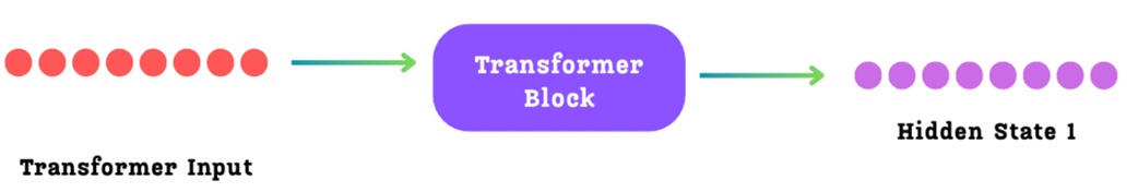
This is a crucial step. It’s not a simple linear transformation; it’s a full, deep computation involving multi-head attention and a feed-forward network. This allows the model to perform complex reasoning about the combination of the previous hidden state and the next token’s embedding, effectively asking, “Given my understanding so far (hᵢᵏ⁻¹), and knowing that the next word is tᵢ₊ₖ, what is my new, updated understanding?”
The output of this Transformer block is the new, refined hidden state, hᵢᵏ. This process is described by Equation 22 from the paper.
Figure 5.11 Equation 22 from the DeepSeek V3 paper.

Step 4: Generating Outputs
This new hidden state, hᵢᵏ, now serves two purposes, completing the loop:
- It is passed as an input to the next MTP Module. The h¹ from Head 1 becomes the input hidden state for Head 2. The h² from Head 2 becomes the input for Head 3, and so on. This is the causal link that makes DeepSeek’s MTP implementation sequential and powerful. Crucially, passing the entire refined hidden state provides a rich, contextualized summary of the sequence so far—far more information than a single predicted token ID could. This is the key advantage of DeepSeek’s causal MTP, as it allows each subsequent module to make its prediction based on a much deeper understanding of the evolving context.
- It is also passed to a Shared Un-Embedding Matrix. This is the same final output/logit layer used by the main model and all other MTP heads. This layer projects the hidden state into the full vocabulary space to produce the logits for the k-th future token.
Figure 5.12 The final prediction steps within an MTP module. The new hidden state generated by the MTP Transformer block is passed to a “Shared Un-Embedding Matrix.” This projects the hidden state into the vocabulary space to produce a logits vector, from which the final token for that prediction step is selected.
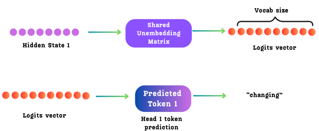
This process is described by Equation 23 from the paper.
Figure 5.13 Equation 23 from the DeepSeek V3 paper.

This formula states that the probability distribution P for the k-th future token is generated by passing the hidden state from the k-th MTP Module through the output head (LitHead).
5.3.3 The final loss calculation
This entire sequential process is performed for each of the D prediction depths. At the end, for a single input token tᵢ, we will have D different predicted tokens. During training, we compare these D predictions to the D actual ground-truth tokens from the input data.
Figure 5.14 The total loss for a single input token is the sum of the individual cross-entropy losses for each of the predicted future tokens.
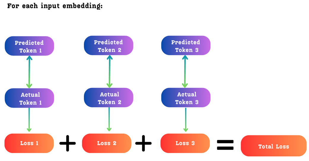
As shown in figure 5.14, the total loss is simply the sum of the individual cross-entropy losses for each prediction depth. This means the model receives a rich, multi-faceted gradient signal, pushing it to become better at not just immediate next-token prediction, but also at longer-term forecasting.
5.4 Implementing a causal multi-token prediction module from scratch
We have now explored the theory behind Multi-Token Prediction, from its core advantages to the specifics of DeepSeek’s advanced causal architecture. While a full, large-scale implementation is deeply integrated into a complex training framework, we can solidify our understanding by building a functional, self-contained version of this mechanism in PyTorch.
This hands-on approach will translate the diagrams and equations we’ve just studied into concrete code. We will build the entire MTP system in stages:
- The MTP Module: The core component that processes one step in the causal chain.
- The Main Model: A wrapper class that integrates the main Transformer trunk and the chain of MTP modules.
- The Forward Pass & Loss: The complete logic for sequential prediction and the combined loss calculation.
Let’s start with the most important new component: the MTP module itself. This class is a direct implementation of the logic shown in Figures 5.9 through 5.13. It takes the hidden state from the previous step and the embedding of the next token, and produces a refined hidden state and a prediction.
We begin by defining two key components. First, we’ll implement RMSNorm, the specific normalization layer used throughout the DeepSeek architecture. This is a foundational utility that ensures numerical stability during training. You can find all imports and helper classes in the chapter’s official GitHub repository.
Listing 5.1 Implementing a Multi-Token Prediction Module from Scratch
class RMSNorm(nn.Module):
    """
    Implements Root Mean Square Layer Normalization.
    """
    def __init__(self, d_model: int, eps: float = 1e-6):
        super().__init__()
        self.eps = eps
        self.weight = nn.Parameter(torch.ones(d_model))

    def forward(self, x: torch.Tensor) -> torch.Tensor:
        # Calculate the inverse square root of the mean of squares
        norm_x = x * torch.rsqrt(x.pow(2).mean(-1, keepdim=True) + self.eps)
        # Apply the learnable weight
        return self.weight * norm_x
Next, we will build the core of the MTP architecture: the DeepSeekMTPModule. It contains a single, dedicated Transformer block and the necessary projection layers. Its purpose is to take the hidden state from the previous step and the embedding of the next token, and produce a refined hidden state for the next step in the causal chain.
Listing 5.2 The Causal MTP Module
class DeepSeekMTPModule(nn.Module):
    def __init__(self, d_model: int, nhead: int, dim_feedforward: int, dropout: float = 0.0):
        super().__init__()
        self.d_model = d_model

        self.projection_matrix = nn.Linear(2 * d_model, d_model, bias=False)  # A

        self.transformer_block = nn.TransformerEncoderLayer(  # B
            d_model=d_model,
            nhead=nhead,
            dim_feedforward=dim_feedforward,
            dropout=dropout,
            activation='gelu',
            batch_first=True,
            norm_first=True
        )

        self.norm_hidden = RMSNorm(d_model) # C
        self.norm_embed = RMSNorm(d_model)

    def forward(self, h_prev: torch.Tensor, future_token_embeds: torch.Tensor) -> torch.Tensor:
        h_normed = self.norm_hidden(h_prev)
        embed_normed = self.norm_embed(future_token_embeds)

        concatenated = torch.cat([h_normed, embed_normed], dim=-1) # D
        h_prime = self.projection_matrix(concatenated)

        h_output = self.transformer_block(h_prime) # E

        return h_output
- A: The projection matrix M_k, which maps the concatenated 2D vector back to the model’s dimension D.
- B: A standard, dedicated Transformer block (TRM_k) for this MTP depth.
- C: Separate RMSNorm layers for the previous hidden state and the future token embedding, as specified in the official formula.
- D: The two normalized inputs are concatenated along the feature dimension.
- E: The projected vector is processed by the Transformer block to produce the new, refined hidden state.
Now that we have the DeepSeekMTPModule building block, we can assemble the full model. The following listing shows the initialization of the DeepSeekV3WithMTP class.
Pay close attention to how the different components are organized. The model contains not just one, but a list of modules_m, one for each prediction depth. It also defines the shared embedding and output layers that will be used by both the main Transformer trunk and all the MTP modules, which is a key aspect of the architecture’s efficiency.
Listing 5.3 Initializing the Full MTP Model Architecture
class DeepSeekV3WithMTP(nn.Module):
    def __init__(
        self,
        vocab_size: int,
        d_model: int,
        num_layers: int,
        nhead: int,
        num_mtp_heads: int,     # D (number of MTP depths) # A
        dim_feedforward: int,
        dropout: float = 0.0,
        mtp_loss_weight: float = 0.1
    ):
        super().__init__()
        # ... (store parameters) ...

        # Shared components used across the model
        self.shared_embed = nn.Embedding(vocab_size, d_model) # B
        self.shared_lm_head = nn.Linear(d_model, vocab_size, bias=False) # C

        # Main transformer backbone (Shared Transformer Trunk)
        self.blocks = nn.ModuleList([ # D
            nn.TransformerEncoderLayer(
                d_model=d_model, nhead=nhead, dim_feedforward=dim_feedforward,
                dropout=dropout, activation='gelu', batch_first=True,
                norm_first=True
            )
            for _ in range(num_layers)
        ])
        self.norm_f = RMSNorm(d_model)

        # Weight tying between embedding and output head
        self.shared_lm_head.weight = self.shared_embed.weight

        # The chain of MTP modules
        self.mtp_modules = nn.ModuleList([ # E
            DeepSeekMTPModule(d_model, nhead, dim_feedforward, dropout)
            for _ in range(num_mtp_heads)
        ])
    # ... (forward method comes next) ...
- A: The parameter num_mtp_heads corresponds to D, the number of future tokens to predict.
- B: The single, shared token embedding layer.
- C: The single, shared output head (un-embedding layer) that projects hidden states to logits.
- D: The main stack of Transformer blocks, referred to as the “Shared Transformer Trunk.”
- E: A list of DeepSeekMTPModule instances, creating the sequential chain for MTP.
With the model structure initialized, we can now implement the forward method. This is where the entire sequential MTP process comes to life. The logic follows a clear sequence:
- The input tokens are first passed through the main Transformer trunk to produce the initial hidden state, main_h.
- The model then enters a loop that iterates through each MTP module in the chain.
- Inside the loop, for each prediction depth k, it uses the hidden state from the previous step (prev_h) and the ground-truth embedding of the k-th future token to generate the new hidden state, curr_h.
- The logits for the k-th future token are computed from curr_h.
- Finally, the total loss is calculated as the sum of the main next-token prediction loss and the weighted average of all the MTP losses.
Listing 5.4 The MTP Forward Pass and Combined Loss Calculation
# ... (inside the DeepSeekV3WithMTP class) ...

    def forward(self, input_ids: torch.Tensor, targets: Optional[torch.Tensor] = None):
        B, S = input_ids.shape
        # ... (other setup) ...

        # --- Main model forward pass ---
        x = self.get_embedding(input_ids)
        # ... (pass through self.blocks) ...
        h_main = self.norm_f(x)
        logits_main = self.get_output_logits(h_main)

        all_logits = [logits_main]
        h_prev = h_main # A

        # --- MTP chain: Sequential prediction ---
        for depth_k in range(1, self.num_mtp_heads + 1):
            L = S - depth_k # B
            if L <= 0: break

            h_prev_sliced = h_prev[:, :L, :] # C

            future_token_ids = input_ids[:, depth_k:depth_k + L]
            future_token_embeds = self.get_embedding(future_token_ids) # D

            h_curr = self.mtp_modules[depth_k - 1](h_prev_sliced, future_token_embeds) # E

            logits_k = self.get_output_logits(h_curr)
            all_logits.append(logits_k)

            h_prev = h_curr # F

        # --- Loss computation ---
        loss = None
        if targets is not None:
            # ... (loss calculation logic) ...
            total_loss = # ... Main model loss ...

            for k, logits_k in enumerate(all_logits[1:], start=1):
                # ... (calculate loss for MTP depth k) ...
                mtp_loss_sum += loss_mtp_k

            # Final loss: L = L_main + (λ/D) * Σ(L_MTP^k)
            if self.num_mtp_heads > 0 and mtp_loss_sum > 0:
                mtp_loss_weighted = (self.mtp_loss_weight / self.num_mtp_heads) * mtp_loss_sum # G
                total_loss += mtp_loss_weighted

            loss = total_loss

        return {"logits_all": all_logits, "loss": loss}
- A: The output of the main trunk serves as the initial hidden state for the MTP chain.
- B: The sequence length L shrinks at each depth k, as there are fewer future tokens to predict.
- C: Slices the previous hidden state to match the current sequence length.
- D: Gathers the ground-truth embeddings for the future tokens at the current depth k.
- E: The core MTP step: the k-1 module is called to produce the new hidden state.
- F: The causal link: the output hidden state becomes the input for the next iteration.
- G: Implements the final loss formula, averaging the MTP losses and scaling by the weight λ.
Listing 5.5 Verifying the Causal MTP Implementation
def verify_deepseek_v3_mtp():
    # --- Model configuration ---
    vocab_size = 1000
    d_model = 128
    num_layers = 6
    nhead = 8
    num_mtp_heads = 3  # D=3 (predict next 3 tokens) # A
    dim_feedforward = 512
    mtp_loss_weight = 0.1

    model = DeepSeekV3WithMTP(
        vocab_size=vocab_size, d_model=d_model, num_layers=num_layers,
        nhead=nhead, num_mtp_heads=num_mtp_heads,
        dim_feedforward=dim_feedforward, mtp_loss_weight=mtp_loss_weight
    )
    print(f"Model created with {sum(p.numel() for p in model.parameters())/1e6:.2f}M params")

    # --- Test data ---
    batch_size = 2
    seq_len = 20
    input_ids = torch.randint(0, vocab_size, (batch_size, seq_len)) # B

    # --- Forward pass and output verification ---
    outputs = model(input_ids, targets=input_ids)
    all_logits = outputs['logits_all']
    loss = outputs['loss']

    print("\nLogits shapes:")
    for i, logits in enumerate(all_logits): # C
        pred_type = "Main" if i == 0 else f"MTP k={i}"
        print(f"  {pred_type:10}: {list(logits.shape)}")

    print(f"\nTotal loss: {loss.item():.4f}") # D
- A: We set the number of MTP heads (prediction depth) to 3.
- B: A dummy batch of input data with a sequence length of 20.
- C: Iterates through the list of output logits to print the shape of each one.
- D: Prints the final, combined loss value.
Running this script produces the following output. Notice how the sequence length (the middle dimension) of the logit tensors decreases by one at each step, confirming our causal chain is correctly implemented.
Model created with 2.01M params

Logits shapes:
  Main      : [2, 20, 1000]
  MTP k=1   : [2, 19, 1000]
  MTP k=2   : [2, 18, 1000]
  MTP k=3   : [2, 17, 1000]

Total loss: 109.1470
With this, we have successfully implemented the core logic of DeepSeek’s Multi-Token Prediction architecture. We’ve seen how a causal chain of dedicated Transformer blocks can be used to predict a horizon of future tokens, providing a richer training signal and a powerful mechanism for better planning and forecasting.
5.5 Quantization: Trading precision for speed and memory
We have now completed our exploration of the high-level architectural pillars of the DeepSeek model: Multi-Head Latent Attention, Mixture of Experts, and Multi-Token Prediction. These innovations define what the model computes. Now, we turn our attention to an equally important topic that defines how these computations are performed with incredible efficiency: FP8 Quantization.
This topic is the final key to understanding how DeepSeek manages to train and run massive, 671-billion-parameter models at a fraction of the cost of its competitors. As we will see, their approach to quantization is a sophisticated, multi-faceted strategy that pushes the boundaries of low-precision training. While “low precision” might sound like a compromise, it is the essential trade-off that unlocks incredible gains in speed and memory efficiency, making large-scale training possible.
We will start by building a solid foundation, understanding what quantization is and why it’s necessary. Then, we will deconstruct the five major innovations that make up DeepSeek’s FP8 training framework.
5.5.1 What is quantization?
At its core, every parameter in a large language model, every weight in every matrix, every bias in every layer is just a number. By default, computers store these numbers with a high degree of precision, typically using a format called 32-bit floating-point (FP32).
Figure 5.15 A visual comparison of a number represented in 32-bit floating-point (FP32) versus 16-bit floating-point (FP16). The diagram illustrates the reduction in the number of bits allocated for the exponent and the mantissa, which results in lower precision and a smaller memory footprint.
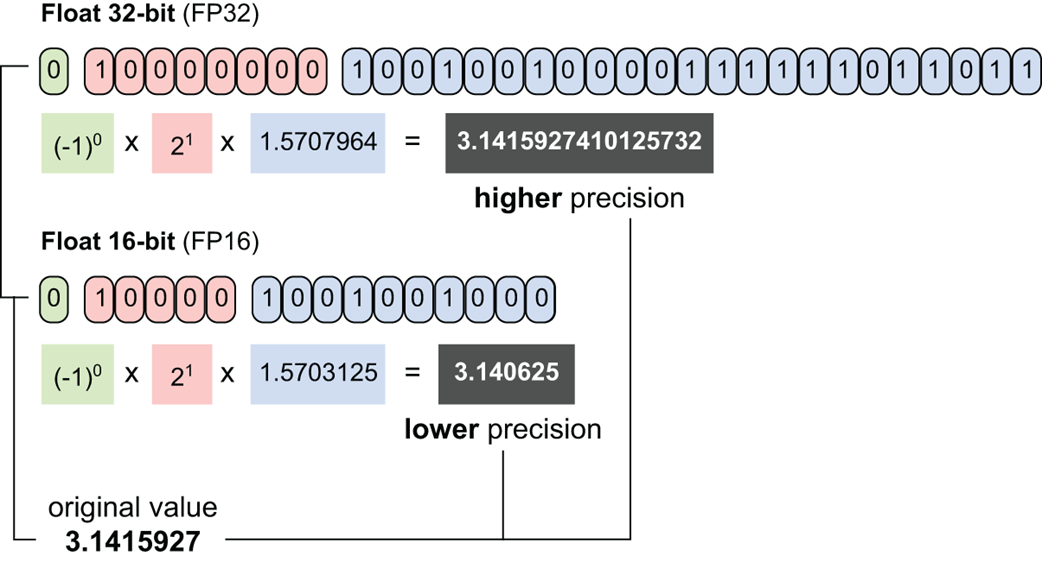
As shown in figure 5.15, an FP32 number uses 32 bits of memory to represent a single value. This allows for very high precision (many decimal places) and a vast dynamic range (the ability to represent both very large and very small numbers).
Quantization is the process of reducing this precision. It is a technique for converting a model’s parameters from a higher bit-width to a lower bit-width. For example, we might quantize a model from FP32 to FP16, meaning every parameter now only uses 16 bits of memory instead of 32.
The intuition behind this is best understood with an analogy.
Figure 5.16 The quantized image uses far fewer colors (less information/precision) but still effectively represents the original image.
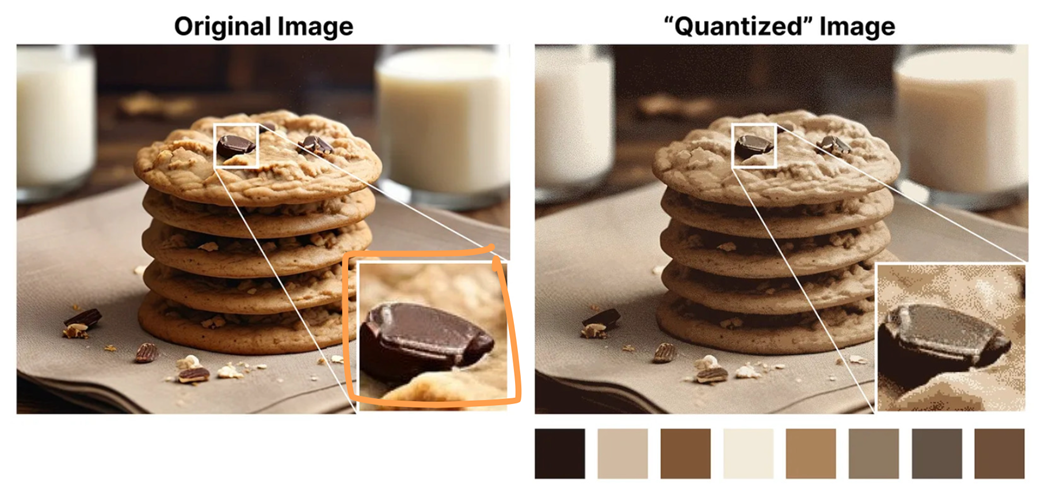
As illustrated in figure 5.16, the original image uses a vast palette of colors to represent every detail with perfect fidelity. The quantized image uses only a small, limited palette of 8 colors. While a close-up inspection reveals a loss of detail (pixelation), the overall image is still clearly recognizable.
Quantization does the same thing to a neural network. It reduces the “palette” of numbers the model can use. While this results in a slight loss of precision for each individual parameter, the overall performance of the model often remains remarkably robust.
5.5.2 Why quantize? The memory cost of high-precision parameters
The primary motivation for quantization is to solve the enormous memory and computational costs associated with large language models. Storing billions of parameters in high precision is incredibly expensive.
Figure 5.17 The memory savings from quantization for a 70-billion parameter model. The calculations demonstrate how reducing the numerical precision from 64-bits to 32-bits, and further to 16-bits, dramatically decreases the total memory required to store the model’s weights.
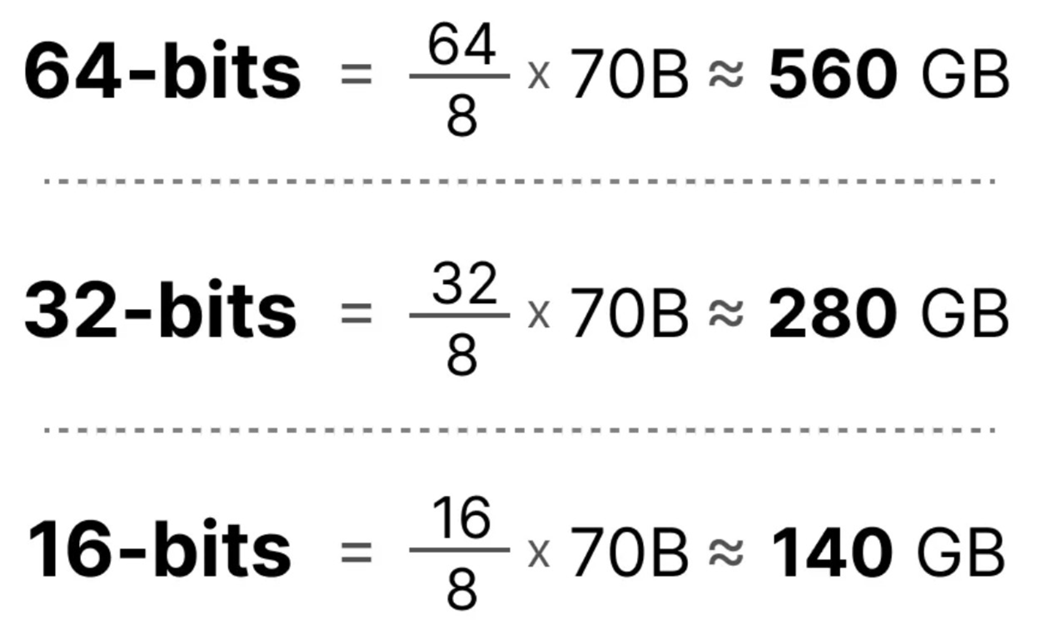
As figure 5.17 shows, the memory savings are dramatic. By quantizing a 70B parameter model from 32-bit to 16-bit, we cut its memory requirement in half, from a staggering 280 GB down to a more manageable 140 GB. This reduction in memory has two direct benefits:
- Faster Training and Inference: Smaller parameters mean less data needs to be moved from the GPU’s main memory to its compute cores, which significantly speeds up every calculation.
- Accessibility: It allows larger models to be run on hardware with less memory.
This is the central bargain of quantization: we trade a small, often acceptable, amount of precision for a massive gain in memory efficiency and computational speed.
5.5.3 Understanding numerical formats: The building blocks of quantization
To understand the specifics of DeepSeek’s framework, we first need to be familiar with the different “palettes” of numbers, or numerical formats, that are commonly used in deep learning. Every floating-point number is represented in memory using three distinct parts:
- Sign (1 bit): The simplest part. This single bit determines if the number is positive (0) or negative (1).
- Exponent: These bits determine the number’s magnitude or dynamic range. They control how large or small the number can be by defining the position of the decimal point (in binary). More exponent bits mean the format can represent a vastly wider range of numbers (e.g., from very close to zero to extremely large).
- Mantissa (or Significand): These bits determine the number’s precision. They represent the actual digits of the number. More mantissa bits mean the format can store more significant digits, resulting in higher precision and smaller gaps between representable numbers.
Let’s see how these components are balanced in the most common formats.
FP32 (32-bit Floating-Point)
This is our high-precision baseline. It uses 1 sign bit, 8 exponent bits, and 23 mantissa bits. Its massive number of mantissa bits gives it very high precision, and the 8 exponent bits give it a vast dynamic range.
FP16 (16-bit Floating-Point)
This was one of the first popular formats for reducing memory. It uses 1 sign bit, 5 exponent bits, and 10 mantissa bits.
Figure 5.18 A comparison of FP32 and FP16.
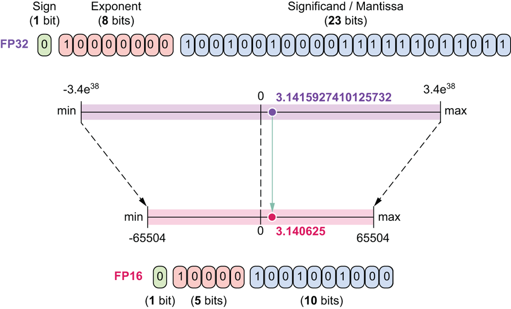
As shown in figure 5.18, FP16 drastically reduces the number of bits for both the exponent and the mantissa. As a result, both its range and precision are significantly smaller than FP32. While memory-efficient, it can sometimes suffer from overflow (numbers becoming too large for its limited exponent) or underflow (numbers becoming too small and losing detail).
BF16 (16-bit “Brain Float”)
This is a clever format developed by Google to get the best of both worlds for training. It uses 1 sign bit, 8 exponent bits, and 7 mantissa bits.
Figure 5.19 A comparison of FP32 and BFloat16.
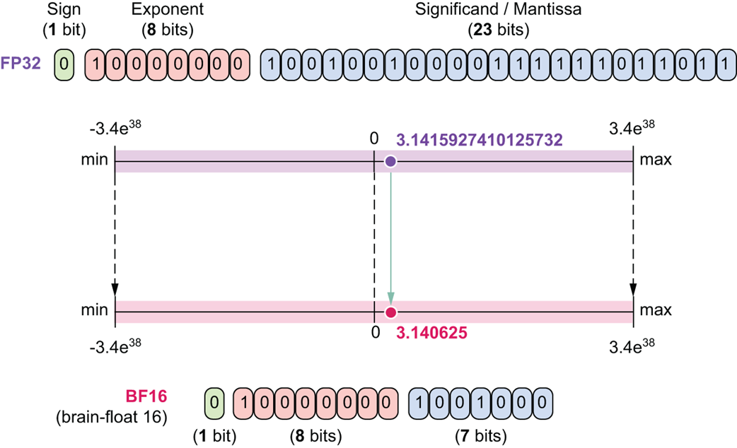
As figure 5.19 shows, BF16 uses the same 8 exponent bits as FP32, giving it the same massive dynamic range. It saves memory by reducing the mantissa to just 7 bits, which means it has lower precision than even FP16. This format is excellent for training because its wide range makes it very resistant to overflow issues.
INT8 (8-bit Integer)
This is an even more aggressive quantization format. It uses 1 sign bit and 7 bits for the value, with no decimal precision.
Figure 5.20 A comparison of FP32 and INT8.
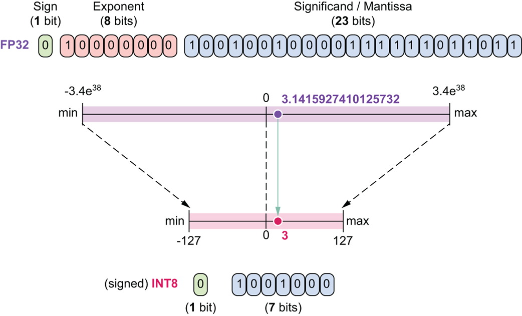
As figure 5.20 illustrates, its range is extremely small, from -127 to 127. While highly efficient, converting to INT8 can lead to a more significant loss of information if the original numbers have a wide range.
FP8 (8-bit Floating-Point)
Finally, the format at the heart of DeepSeek’s strategy is FP8. It’s an 8-bit format that, unlike INT8, still retains a sign, exponent, and mantissa (e.g., E4M3 with 4 exponent bits and 3 mantissa bits). It offers a compromise between the extreme efficiency of INT8 and the flexibility of floating-point numbers.
5.5.4 The basic mechanism: Scaling
How do we actually convert a vector of high-precision FP32 numbers into a lower-precision format like INT8? The process is called scaling. The core idea is to map the range of our original numbers onto the target range of the new format without losing the relative relationships between them.
Figure 5.21 The scaling process for quantization. The original range of the FP32 tensor is mapped to the target range of the INT8 format.
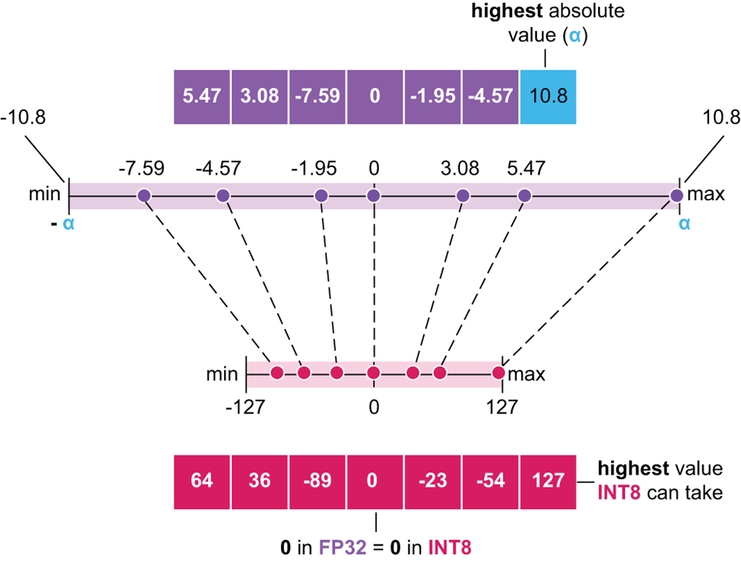
As illustrated in figure 5.21, the process involves a few simple steps:
- Find the Maximum Absolute Value (α): We first scan our entire input vector (or tensor) and find the number with the largest absolute value. In this example, it’s 10.8. This value, α, defines the effective range of our original data, from -α to +α.
- Calculate the Scaling Factor: We want to map this original range to the target range of the INT8 format, which is -127 to 127. The scaling factor is simply target_range_max / original_range_max, which is 127 / 10.8.
- Quantize: We multiply every number in our original vector by this scaling factor and then round to the nearest integer. For example, the number -7.59 becomes round(-7.59 * (127 / 10.8)), which results in -89. This new integer is the quantized representation.
- De-quantize: To recover the original numbers for use in a computation (with some precision loss), we would simply perform the inverse operation: divide the quantized integer by the same scaling factor. For example, -89 / (127 / 10.8) gives us approximately -7.59.
This concept of finding a scaling factor based on the maximum value in a tensor is the most important prerequisite for understanding the advanced techniques used by DeepSeek. As we will see, their first major innovation, fine-grained quantization, is a clever new way of applying this fundamental scaling principle.
5.5.5 The five pillars of DeepSeek’s FP8 training
Now that we have a solid foundational understanding of what quantization is and the different numerical formats involved, we can dive into the specifics of DeepSeek’s implementation. Their approach is not a single technique but a sophisticated, multi-faceted framework composed of five key innovations that work together to enable stable and efficient training in the ultra-low FP8 precision.
These five pillars are:
- The Mixed Precision Framework
- Fine-Grained Quantization
- Increasing Accumulation Precision
- Mantissa Over Exponents
- Online Quantization
Let’s deconstruct each of these pillars one by one, explaining the problem they solve and how they are implemented, both visually and mathematically.
5.5.6 Pillar 1: The mixed precision framework
The first and most fundamental pillar of DeepSeek’s strategy is the Mixed Precision Framework.
The Core Idea: Not All Numbers are Created Equal
The central insight behind mixed precision is that not all operations or stored values in a neural network require the same level of numerical precision. It would be inefficient to use a 32-bit number with many decimal places for a value that doesn’t need it, just as it would be a mistake to use a low-precision number for a value that is highly sensitive to small errors.
A mixed precision framework, therefore, is a strategic system that uses different numerical formats for different parts of the training process. The goal is to get the best of both worlds:
- Use low-precision formats (like FP8) for the vast majority of computations (like massive matrix multiplications) to maximize speed and minimize memory usage.
- Use high-precision formats (like FP32) for the most sensitive and critical components (like updating the model’s master weights) to ensure the training process remains stable and accurate.
DeepSeek’s framework is a masterclass in intelligently balancing these trade-offs. Let’s walk through how it handles the different operations in a standard linear layer during a full forward and backward pass.
Figure 5.22 The mixed precision framework with FP8 data format in the Linear operator. The diagram illustrates the flow of data through a linear layer, showing how inputs and weights are converted to low-precision FP8 for fast computation, while critical components like master weights and gradients are maintained in high-precision FP32 for stability.
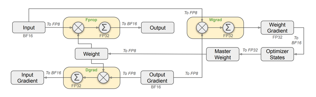
This diagram looks complex, but it simply visualizes the flow of data through the four key stages of a linear layer’s computation. Let’s break down each stage.
A. Forward Propagation (Fprop)
The forward pass is the standard prediction step, where output = weights * input. This is the primary computation that happens during inference.
Figure 5.23 The data flow and precision formats for the forward pass.
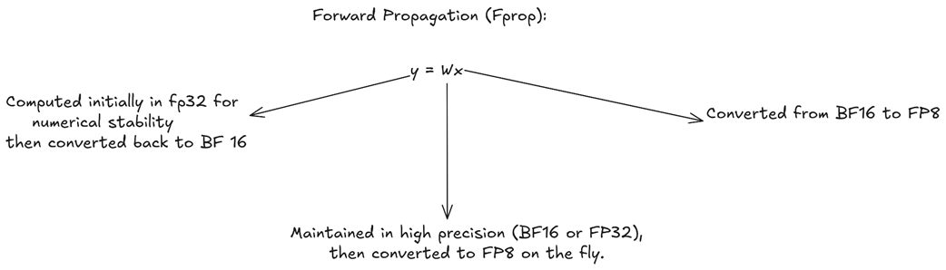
As shown in figure 5.23, a strategic mix of precisions is used:
- Inputs (x): The input activations from the previous layer are typically stored in BF16. For the actual multiplication, they are converted on-the-fly to the highly efficient FP8 format.
- Weights (W): The main “master” copy of the weights is maintained in high-precision FP32 (or BF16). For the multiplication, these weights are also converted on-the-fly to FP8.
- Output (y): The result of the FP8 x FP8 multiplication is accumulated in full FP32 to prevent numerical errors and maintain stability. This high-precision result is then immediately converted back down to BF16 for storage in memory.
Why this mix? The heavy matrix multiplication is done in the fastest, lowest-precision format (FP8), while the final result is accumulated and stored in higher-precision formats to prevent the loss of information.
B. Backward Propagation: Gradient with respect to Inputs (Dgrad)
After the forward pass, the model calculates its error, and the learning process begins. Backward propagation involves calculating the gradients of the signals that tell each weight how to update itself to reduce the error. This process is more complex and involves calculating two primary gradients for our y = Wx layer: the gradient with respect to the inputs (dgrad) and the gradient with respect to the weights (wgrad).
Figure 5.24 The data flow for the Dgrad calculation.
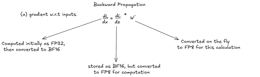
The gradient with respect to the input, dL/dx, is needed to continue the backpropagation process to the previous layer. It’s calculated using the chain rule:
\[dL/dx = (dL/dz) * W^T\]Here, dL/dz is the gradient coming from the next layer, and W^T is the transpose of the weight matrix. DeepSeek applies a similar mixed precision strategy here:
- The incoming gradient (dL/dy), stored as BF16, is converted to FP8 for the computation.
- The original weight matrix (W), which is in high precision, is also converted on the fly to FP8 for this calculation.
- The resulting gradient, dL/dx, is computed with an FP32 accumulator and then stored as BF16 to be passed back to the previous layer.
Notice the symmetry with the forward pass: the core operation is FP8 for speed, but the result that gets passed between layers is kept in the more stable BF16 format.
C. Backward Propagation: Gradient with respect to Weights (Wgrad)
Figure 5.25 The data flow for the Wgrad calculation.
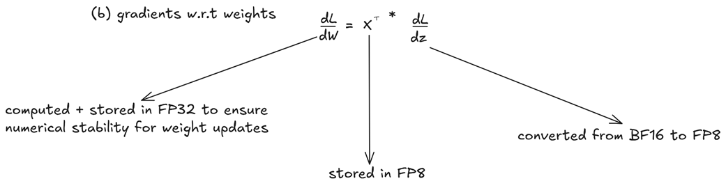
This is the most critical gradient, as it will be used to update the model’s actual knowledge. The gradient dL/dW tells the model how to adjust its weights. It is calculated as:
\[dL/dW = x^T * (dL/dz)\]Here, the precision strategy changes to prioritize accuracy. A noisy or imprecise weight gradient can destabilize the entire training process. Therefore, DeepSeek makes a crucial decision:
- The input to the layer (x), which was stored in FP8 during the forward pass, is used here.
- The incoming gradient (dL/dy) is converted from BF16 to FP8.
- The resulting weight gradient, dL/dW, is computed and, most importantly, stored in full FP32 precision.
This is a key part of the “mixed” precision framework. While other gradients can be stored in BF16, the weight gradient is kept at the highest fidelity to ensure that the updates to the model’s core parameters are as accurate as possible.
D. The Weight Update
Figure 5.26 The weight update step is performed entirely in high-precision FP32.
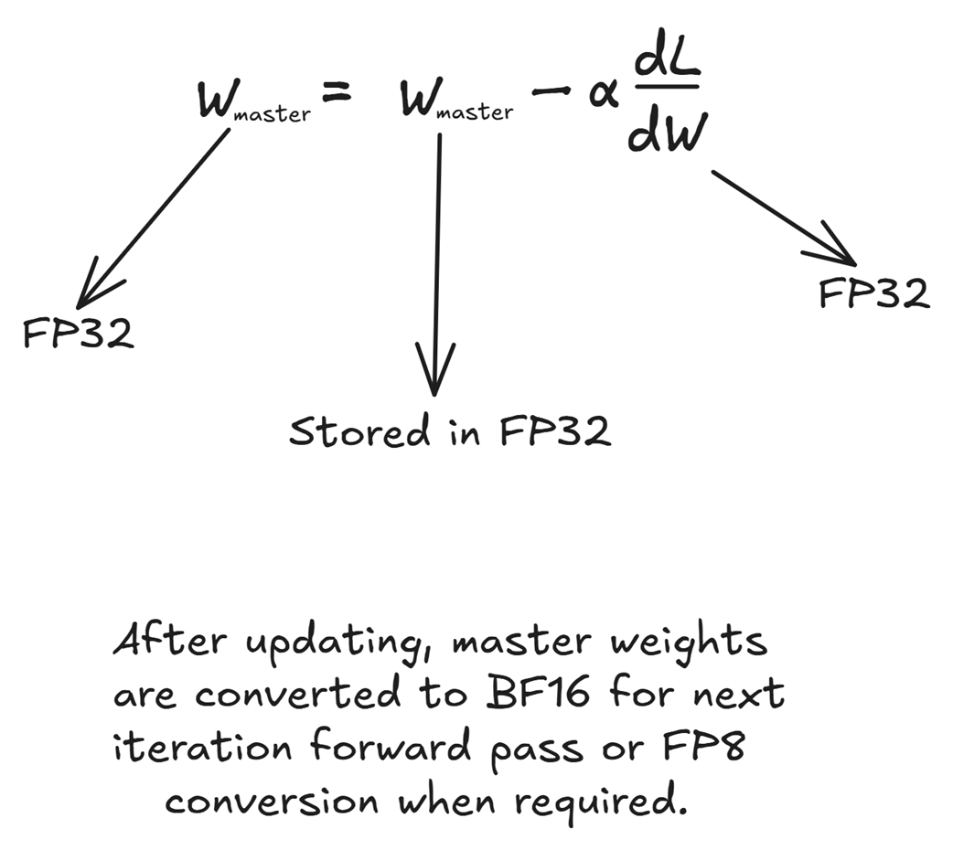
Finally, the optimizer uses the high-precision weight gradient to update the master weights.
\[W\_master\_new = W\_master\_old - learning\_rate * (dL/dW)\]Because this step directly modifies the model’s permanent knowledge, stability is paramount. Therefore, all components of this operation are maintained in FP32:
- The master weights are stored in FP32.
- The weight gradients (dL/dW) are already in FP32.
- The optimizer’s internal states (like momentum and variance in AdamW) are also kept in FP32.
The entire update happens in high precision. After the W_master_new is computed, this FP32 version is stored. For the next training iteration’s forward pass, these master weights will once again be converted on the fly to FP8, completing the cycle.
By converting inputs and weights to FP8 for all three major GEMM (General Matrix Multiplication) operations (Fprop, Dgrad, Wgrad), DeepSeek maximizes the throughput and leverages the full power of modern hardware. This provides up to a 2x speed improvement over BF16 operations.
They identified the most sensitive parts of the training loop. The master weights and optimizer states are kept in FP32 to prevent error accumulation and ensure stable learning. Inter-layer activations and gradients (y and dL/dy) are kept in BF16, providing a robust middle ground that is more memory-efficient than FP32 but safer than FP8.
DeepSeek’s team went even further. They identified that certain modules in the Transformer architecture are more sensitive to quantization errors than others. As a result, they chose to keep these specific modules in higher precision (BF16), completely bypassing the FP8 quantization for them. These sensitive components include:
- The Embedding Modules (both token and positional)
- The final Output Head (which projects to the vocabulary)
- Mixture-of-Experts (MoE) Gating Modules
- Normalization Layers (e.g., RMSNorm)
- Attention Operators (specifically, the softmax and context vector calculation)
This balance of high-speed, low-precision computation with high-precision storage for critical components allows DeepSeek to train massive models faster and with less memory, without succumbing to the instability that plagues naive low-precision training approaches. It is the bedrock upon which the other four pillars of their FP8 framework are built.
5.5.7 Pillar 2: Fine-grained quantization
The Mixed Precision Framework defines which numerical formats to use for specific operations within the model. The second pillar, Fine-Grained Quantization, addresses how to convert numbers from a high-precision format like BF16 to a low-precision format like FP8 in a way that preserves as much information as possible.
As we covered in section 5.5.4, the standard mechanism for this conversion is scaling. We find the maximum absolute value in an entire tensor, and we use that value to scale every single number in the tensor into the target range (e.g., the range of FP8), but it does come with one problem.
The problem with outliers in standard quantization
This standard, tensor-wise scaling approach has a major weakness: it is extremely sensitive to outliers. Even a single large value in a massive tensor can drastically reduce the precision for all other values.
Let’s illustrate this with a concrete numerical example. Imagine we have a small vector of activation outputs that we want to quantize to an 8-bit integer format (range -127 to 127): [2.0, 3.0, 500.0]. The presence of the 500.0 outlier completely corrupts the precision of the other values:
- Find Max Absolute Value (α): The maximum absolute value is α = 500.0.
- Calculate Scaling Factor (s): To map the range [-500, 500] to [-127, 127], our scaling factor is s = 127 / 500 = 0.254.
- Quantize: We multiply each element by s and round to the nearest integer:
- round(2.0 * 0.254) = round(0.508) = 1
- round(3.0 * 0.254) = round(0.762) = 1
- round(500.0 * 0.254) = round(127.0) = 127
- The resulting quantized vector is [1, 1, 127]. The crucial distinction between 2.0 and 3.0 has been completely erased.
- De-quantize: When we convert back by dividing by s, we get [1/0.254, 1/0.254, 127/0.254], which is approximately [3.94, 3.94, 500.0].
The relative error for the first two values is catastrophic (97% and 31% respectively), while the outlier is recovered almost perfectly. This is a critical problem in large language models, where activation values can have enormous dynamic ranges.
The DeepSeek solution: Grouping for separate scaling
To solve this, DeepSeek implemented a technique called Fine-Grained Quantization. The idea is brilliantly simple: if a single scaling factor for the whole tensor is problematic, why not break the tensor into smaller chunks and use a separate scaling factor for each chunk independently?
Instead of calculating one maximum value for the entire tensor, DeepSeek divides the tensor into smaller chunks (or “groups” or “tiles”) and calculates a separate scaling factor for each chunk independently. This strategy is applied differently for activations and weights, the two inputs to our core matrix multiplication operation.
Fine-Grained quantization for activations (inputs)
First, let’s consider the activations, which are the input vectors to a given layer. An activation vector in a large model can be very long (e.g., with a dimension of 7168 in DeepSeek-V3). To quantize it, DeepSeek breaks it down into smaller, contiguous groups.
Figure 5.27 Fine-Grained Quantization for an activation vector. The vector is partitioned into smaller groups. Each group is scaled independently based on the maximum value within that group, preserving precision for values in groups that do not contain large outliers.
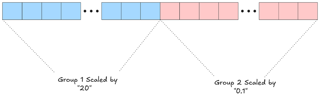
As figure 5.27 illustrates, an outlier in one group no longer affects the others. Let’s say Group 1 contains values with a maximum of “20”, while Group 2 contains much smaller values with a maximum of “0.1”. With fine-grained quantization:
- All elements in Group 1 are scaled by 20.
- All elements in Group 2 are scaled by 0.1.
The small values in Group 2 are now scaled appropriately, preserving their relative differences and ensuring they are not “squashed” down to near-zero by the outlier in Group 1. This per-group scaling is crucial for maintaining the fidelity of the model’s internal representations. In their implementation, DeepSeek uses a group size (Ng) of 128 elements for activations, meaning every 128 channels of an activation vector get their own private scaling factor.
Fine-grained quantization for weights
A similar principle applies to the weight matrices, but adapted for their two-dimensional structure. A large weight matrix is not treated as one monolithic block. Instead, it is partitioned into smaller 2D “tiles” or “blocks.”
Figure 5.28 Fine-Grained Quantization for a weight matrix. The matrix is divided into smaller blocks (e.g., W₁₁, W₁₂, etc.), and each block is quantized independently with its own unique scaling factor.

As shown in figure 5.28, a matrix W might be broken into four blocks: W₁₁, W₂₁, W₁₂, and W₂₂. Each of these blocks is quantized completely independently:
- W₁₁ is scaled by Scaling Factor 1, based on its own internal max value.
- W₂₁ is scaled by Scaling Factor 2, based on its max value.
- …and so on for all blocks.
This block-wise approach for weights ensures that if a few parameters in one region of the matrix learn very large values, they do not degrade the precision of the millions of other weights in the remaining blocks. For their FP8 framework, DeepSeek uses a block size of 128x128.
The full mechanism in action
Now we can understand the complete flow diagram presented by the DeepSeek team. It visualizes how these two fine-grained inputs come together.
Figure 5.29 The complete Fine-Grained Quantization workflow.
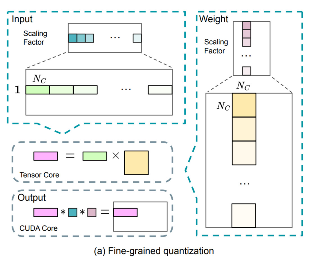
- Input (Activations): The input vector is shown on the top-left. It’s partitioned into chunks of size Ks. A unique Scaling Factor (represented by the different shades of green/teal) is calculated for each chunk.
- Weight: The weight matrix is shown on the top-right. It’s partitioned into blocks of Ks (in this case, Ks x Ks). Each block gets its own Scaling Factor (shades of purple/pink).
- Tensor Core Computation: The core matrix multiplication (Output = Input × Weight) is performed on the specialized, high-speed Tensor Cores. This operation takes the quantized FP8 values as input and produces a low-precision intermediate output (pink rectangle).
- CUDA Core De-quantization: The final step happens on the general-purpose CUDA Cores. The low-precision output from the Tensor Core is de-quantized. This is done by multiplying it with the corresponding scaling factors from both the input and the weights to restore its original magnitude (albeit with some precision loss). This final, high-precision output is then ready for the next stage of the framework.
By breaking down the quantization process into fine-grained, independent chunks, DeepSeek ensures that the numerical precision is maintained at a local level, making the entire training process far more robust to the volatile and high-dynamic-range values that are common in LLMs. This simple “divide and conquer” strategy is one of the key enablers of stable FP8 training at scale.
5.5.8 Pillar 3: Increasing accumulation precision
The third pillar addresses a subtle but critical hardware limitation in modern GPUs. While GPUs are exceptionally good at performing low-precision matrix multiplications (like FP8 x FP8), there’s a limit to the precision they use for the intermediate results during the multiplication process itself.
The problem: Losing precision in the accumulator
Let’s revisit the matrix multiplication Y = WX. To compute a single element in the output matrix Y, we perform a dot product: we multiply corresponding elements from a row of W and a column of X, and then sum (or accumulate) all those products together.
\[Y\_ij = W\_i1*X\_1j + W\_i2*X\_2j + ... + W\_ik*X\_kj\]When W and X are in FP8, each individual product (W_ik*X_kj) is computed. The GPU’s specialized hardware, called Tensor Cores, then needs to add these products up. The internal memory register that holds this running sum is called an accumulator.
The problem is that on modern hardware like NVIDIA’s H800 GPUs, this internal accumulator has limited precision (e.g., around 14 bits), which is significantly lower than the standard 32-bit (FP32) precision. If the inner dimension k of the matrix multiplication is very large (e.g., 4096 or more, which is common in LLMs), we are summing up thousands of these small products. If the accumulator doesn’t have enough precision, we can encounter underflow issues, where the intermediate sum is too small to be accurately represented, and the final result can have significant numerical errors, potentially as high as 2%. This can severely impact the model’s accuracy.
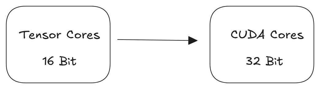
The DeepSeek solution: Promotion to CUDA Cores
To solve this problem, DeepSeek implemented a strategy called promotion to CUDA Cores. The core idea is to leverage the two different types of computational units available on modern GPUs. Tensor Cores are highly specialized, designed to perform matrix multiplication at incredible speeds but with limited precision. In contrast, CUDA Cores are the general-purpose workhorses of the GPU, capable of running a wide variety of tasks with full, high precision, albeit more slowly.
DeepSeek’s strategy is to periodically move the intermediate accumulation results from the fast, low-precision Tensor Cores to the flexible, high-precision CUDA Cores, which can then perform the final accumulation in full FP32 precision.
Figure 5.30 The core strategy for increasing accumulation precision: intermediate results are periodically moved from the low-precision environment of the Tensor Cores to the high-precision environment of the CUDA Cores.
To truly understand this mechanism, we need to look closer at the specific hardware components involved. The calculation begins within the Tensor Core, which performs high-speed, low-precision multiplications in small bursts using an instruction called MMA (Matrix-Multiply-Accumulate).
During each MMA step, the intermediate results are accumulated in a low-precision register, labeled “Low Prec Acc” in the diagram (figure 5.30). The challenge is that this accumulator has limited precision. DeepSeek’s innovation is to not wait until the entire calculation is finished. Instead, at a fixed interval (Nc), the partial sum from the “Low Prec Acc” is periodically “promoted” or transferred to a general-purpose CUDA Core.
The CUDA Core takes this partial sum and adds it to an “FP32 Register,” which has full high-precision capabilities. By performing the final accumulation in this high-precision register, DeepSeek significantly reduces the risk of the underflow issues that plague standard low-precision accumulation, ensuring numerical stability.
Figure 5.31 The Increasing Accumulation Precision mechanism in detail. Low-precision accumulation happens in bursts on the Tensor Core, and results are periodically promoted to a high-precision FP32 register on the CUDA Core.
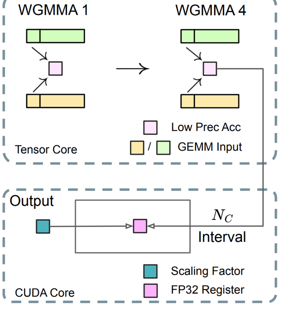
Let’s trace the journey of the data through this diagram step-by-step, identifying every component:
Part 1: The tensor core: High-speed, low-precision work
The top section of figure 5.31, labeled “Tensor Core,” shows where the bulk of the raw computation happens.
- GEMM Inputs: These are the two rectangular blocks at the very top representing the inputs to our matrix multiplication, y = Wx. One block represents the input tensor (e.g., the fine-grained activation vector), and the other represents the weight matrix. Both are already in the fast FP8 format.
- MMA (Matrix-Multiply-Accumulate): This is a highly optimized, low-level NVIDIA instruction that tells a group of GPU threads (a “warp”) to perform a chunk of a matrix multiplication. You can think of MMA 1 through MMA 4 as sequential steps in a much longer dot product. For instance, MMA 1 might compute the sum of the first 32 products in our Y_ij equation.
- Low Prec Acc: This is the small square register labeled “Low Prec Acc,” representing the Low Precision Accumulator. It’s an internal hardware register within the Tensor Core that holds the running sum. In MMA 1, the first set of products is calculated and stored here. In the next step of the MMA sequence, the next set of products would be calculated and added to this same accumulator. The key point is that this register has limited precision (around 14 bits).
Part 2: The bridge: Periodic promotion to high precision
The crucial innovation is the arrow that connects the Tensor Core to the CUDA Core. This is not a one-time data transfer at the end of the calculation; it is a periodic promotion.
Nc Interval: DeepSeek does not wait for all steps of the MMA to complete. Instead, after a fixed interval of Nc element-wise operations (the paper specifies Nc = 128), the process is paused. The partial sum that has been calculated and stored in the “Low Prec Acc” register is copied out of the Tensor Core.
Part 3: The CUDA Core: Low-speed, high-precision finishing
The bottom section of the diagram, labeled “CUDA Core,” is where the final, numerically stable part of the process occurs. CUDA Cores are the GPU’s general-purpose workhorses, capable of handling full FP32 operations.
FP32 Register (Light Blue Square): The partial sum from the Tensor Core arrives and is placed into a register that can store a full 32-bit floating-point number. This register has ample precision to hold the sum of thousands of products without any risk of underflow or precision loss. As more partial sums arrive every Nc interval from the Tensor Core, they are safely added to this high-precision running total.
Scaling Factor (Teal Boxes): At the same time, the CUDA Core can efficiently handle the de-quantization. It takes the Scaling Factors that were calculated during the Fine-Grained Quantization step (Pillar 2) and multiplies them with the high-precision accumulated value.
Output: The final result is a de-quantized, high-precision value that is numerically stable and ready to be stored as BF16 for the next layer in the network.
This hybrid approach perfectly embodies the “best of both worlds” philosophy. It uses the right tool for the right job—fast, specialized Tensor Cores for the bulk of the multiplications and slower, general-purpose CUDA Cores for the final, high-precision accumulation and de-quantization. This synergy allows DeepSeek to achieve both the incredible speed of FP8 computation and the numerical accuracy of FP32 accumulation.
5.5.9 Pillar 4: Mantissa over exponents
As we discussed in section 5.5.3, any floating-point format is a trade-off between the number of bits allocated to the exponent (which determines the dynamic range) and the mantissa (which determines the precision).
For the 8-bit FP8 format, two main standards have emerged:
- E5M2: Uses 5 bits for the exponent and 2 bits for the mantissa. This format has a larger dynamic range (it can represent a wider span of numbers) but lower precision.
- E4M3: Uses 4 bits for the exponent and 3 bits for the mantissa. This format has a smaller dynamic range but higher precision.
The conventional approach
Prior to DeepSeek, a common strategy in mixed-precision training was to use a hybrid approach:
- Use the high-precision E4M3 for the forward pass (Fprop), where the values are more controlled.
- Use the high-range E5M2 for the backward pass (Dgrad and Wgrad), as gradients can sometimes have very large values (outliers) that could cause an overflow in the smaller range of E4M3.
DeepSeek implementation: Uniform E4M3
The DeepSeek team argued that this hybrid approach was a workaround for a problem they had already solved. Thanks to their Fine-Grained Quantization (Pillar 2), the problem of outliers is significantly mitigated.
Because they are scaling activations and weights in small, independent blocks, a large outlier in one block does not affect the scaling of the others. This prevents the “squashing” of values that would normally lead to precision loss. The fine-grained scaling factors effectively manage the dynamic range at a local level.
This insight allowed them to make a powerful simplification: they chose to use the higher-precision E4M3 format uniformly for all operations, including both the forward and backward passes.
By relying on their fine-grained quantization to handle the dynamic range, they could consistently use the format with more mantissa bits, thereby preserving a higher level of precision throughout the entire training process. The DeepSeek paper notes:
“By operating on smaller element groups, our methodology effectively shares exponent bits among these grouped elements, mitigating the impact of the limited dynamic range.”
This is a subtle but important innovation. It demonstrates how DeepSeek’s different quantization techniques work together synergistically. The strength of their fine-grained scaling allowed them to make a more aggressive choice in favor of precision, which is a key contributor to the stability and performance of their FP8 training framework.
5.5.10 Pillar 5: Online quantization
The final piece of DeepSeek’s quantization puzzle addresses the question of when the scaling factors are calculated. As we know, the scaling factor is derived from the maximum absolute value of a tensor. But which tensor? The one from the previous step, or the one we are currently processing?
The conventional approach: Delayed quantization
Many quantization frameworks use a technique called Delayed Quantization. In this approach, the scaling factor used to quantize the current tensor is derived from the maximum value observed in past iterations or batches. It maintains a running history of maximum values and uses that historical information to estimate a good scaling factor for the current step.
The problem with this approach is that the data distribution can change rapidly during training. The maximum value in the current batch might be significantly different from the historical maximum.
- If the current maximum is much larger than the historical one, using the old, smaller scaling factor can lead to overflow, where the quantized values exceed the representable range of FP8.
- If the current maximum is much smaller than the historical one, using the old, larger scaling factor can lead to underflow and a catastrophic loss of precision (the “squashing” problem we saw earlier).
The DeepSeek solution: Online quantization
To solve this, DeepSeek uses Online Quantization. The idea is simple and robust: calculate the scaling factor in real-time, based on the data from the current tensor itself.
Instead of relying on historical information, the workflow is:
- For the current batch of activations or weights, first perform a quick pass to find the maximum absolute value within that specific batch.
- Use this “online” maximum value to derive the scaling factor.
- Apply this fresh, perfectly calibrated scaling factor to quantize the current tensor.
This on-the-fly calculation ensures that the scaling factor is always perfectly tailored to the dynamic range of the data being processed at that exact moment. It completely avoids the risk of overflow or underflow caused by using stale, historical scaling factors.
While this adds a small computational overhead (the initial pass to find the maximum), it’s worth noting that finding the maximum value in a tensor is an order of magnitude faster than the matrix multiplications that form the bulk of the computation. The benefit gained in terms of numerical stability and accuracy is therefore enormous. This commitment to using the most accurate, real-time information possible, even at the cost of a computationally inexpensive pre-pass, is a recurring theme in DeepSeek’s design and is a key reason for the robustness of their FP8 training framework.
In the next chapter, we will apply this knowledge by creating a small-scale, DeepSeek-like model, demonstrating how these concepts come together in practice.
5.6 Summary
- Multi-Token Prediction (MTP) enhances data efficiency by training models to predict a horizon of future tokens simultaneously, providing richer gradient signals for long-range coherence.
- The MTP training objective implicitly assigns higher weight to “choice points” or critical pattern-shifting tokens in a sequence, thereby developing better planning capabilities in the model.
- DeepSeek’s causal MTP implementation sequentially refines a hidden state, where the prediction for one token informs the next, creating a powerful forecasting mechanism.
- Quantization is essential for large-scale training, reducing memory usage and computational cost by converting high-precision parameters to low-precision formats like FP8.
- DeepSeek’s FP8 framework uses a mixed precision strategy, performing core computations in low precision while storing sensitive components, such as master weights and optimizer states, in high precision to ensure numerical stability.
- Fine-Grained Quantization: To mitigate precision loss from outliers, DeepSeek calculates separate scaling factors for small blocks of activations and weights, preserving fidelity at a local level.
- Increasing Accumulation Precision: DeepSeek promotes intermediate results from low-precision Tensor Cores to high-precision CUDA Cores, where accumulation occurs in full FP32 precision to prevent underflow errors.
- Mantissa over Exponents: DeepSeek uniformly uses the higher-precision E4M3 format for both forward and backward passes, enabled by fine-grained quantization, which effectively manages dynamic range.
- Online Quantization: DeepSeek calculates scaling factors in real-time based on the current batch’s data, ensuring accurate scaling and avoiding the instability associated with historical data.