2 Generating Text with a Pre-trained LLM

This chapter covers:

• Setting up the code environment for working with LLMs
• How to use a tokenizer to prepare input text for an LLM
• The step-by-step process of text generation using a pre-trained LLM
• Caching and compilation techniques for speeding up LLM text generation

In the previous chapter, we discussed the difference between conventional large language models (LLMs) and reasoning models. Also, we introduced several techniques to improve the reasoning capabilities of LLMs. These reasoning techniques are usually applied on top of a conventional (base) LLM.

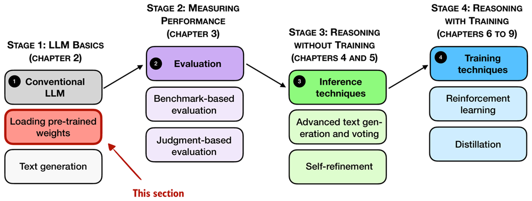
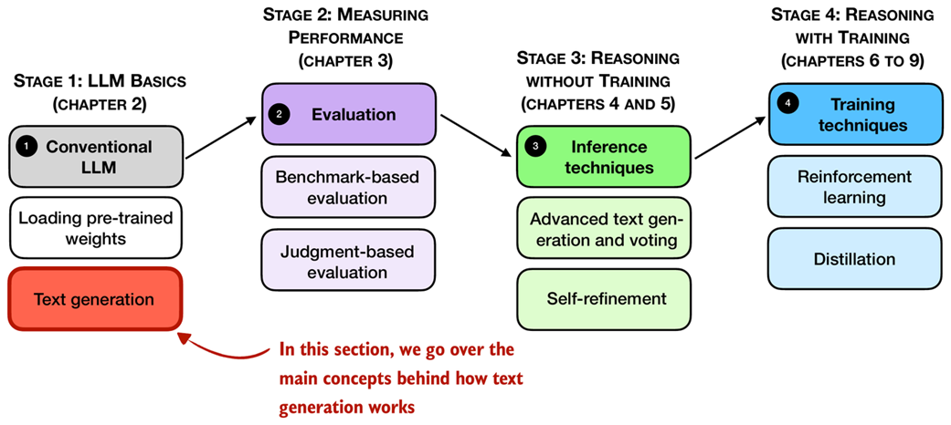
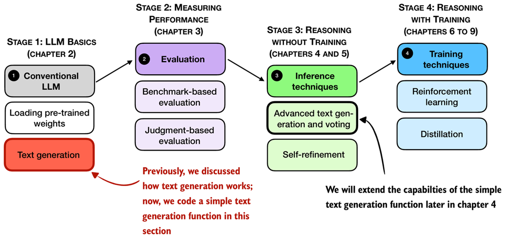
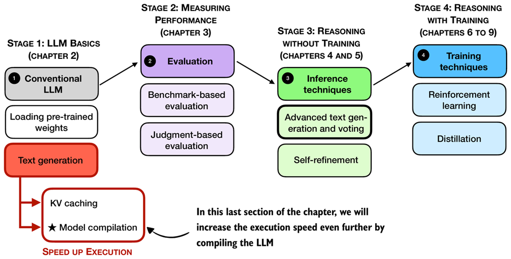
In this chapter, we will lay the groundwork for the upcoming chapters and load such a conventional LLM on top of which we can apply reasoning techniques in subsequent chapters, as illustrated in Figure 2.1. This conventional LLM is an LLM that has already been pre-trained to generate general texts (but it has not been specifically trained or enhanced for reasoning).

Figure 2.1 A mental model depicting the four main stages of developing a reasoning model. This chapter focuses on stage 1, loading a conventional LLM and implementing the text generation functionality.

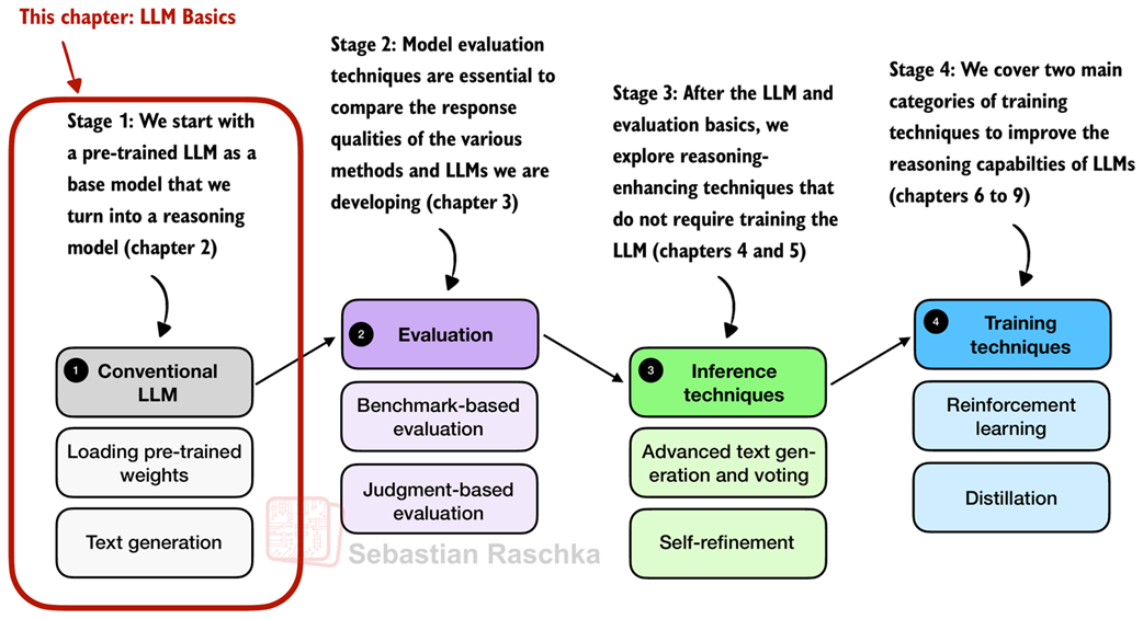
In addition to setting up the coding environment and loading a pre-trained LLM, you will learn how to use a tokenizer to prepare text input for the model. As illustrated in Figure 2.1, you will also implement a text generation function, enabling practical use of the LLM to generate text. This functionality will be used and further improved in later chapters.

2.1 Introduction to LLMs for text generation

In this chapter, we implement all the necessary LLM essentials, from setting up our coding environment and loading a pre-trained LLM to generating text that we will reuse and build upon in this book. In this sense, this chapter can be understood as a setup chapter.

This LLM will be capable of following basic instructions and generating coherent text, as illustrated in Figure 2.2.

Figure 2.2 An overview depicting an LLM generating a response (output text) given a user query (input text).

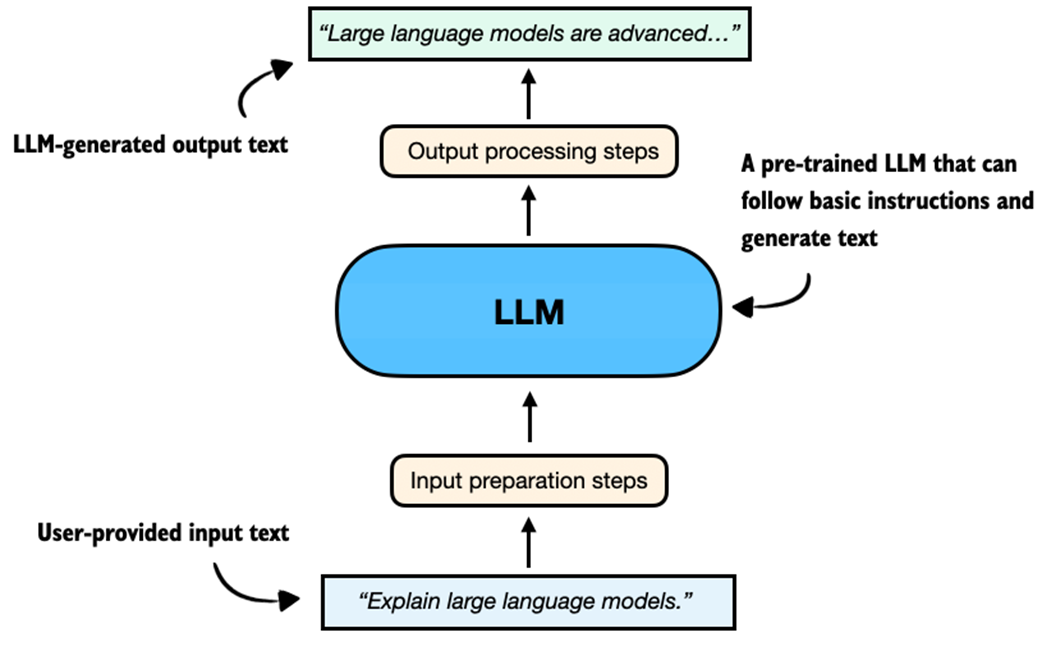
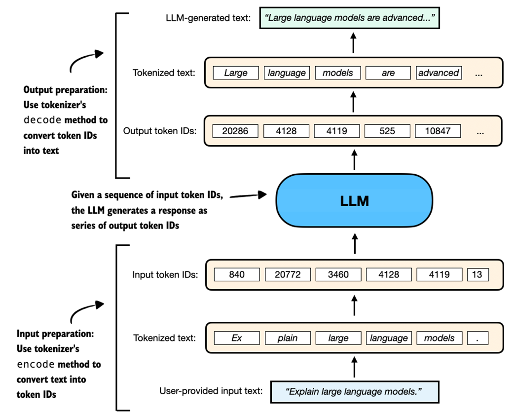
Figure 2.2 summarizes the components of an LLM text generation pipeline, and we will discuss and implement these steps in more detail later in this chapter.

Note: By convention, diagrams involving neural networks such as LLMs are drawn and read vertically from bottom (inputs) to top (outputs). Arrows indicate the flow of information upward through the model.

If you have not coded an LLM or used LLMs programmatically before, this chapter will teach you how the text generation process works. However, in this chapter, we will not go deep into the internals of an LLM, such as the attention mechanism and other architectural components; this is the topic of my other book, Build a Large Language Model (From Scratch). Note that understanding these internals is not required for this book, and, if you are curious, you can learn about them after you finish reading this book.

This chapter will also be helpful if you have already read the earlier Build a Large Language Model (From Scratch) book, since it adds new material on speeding up inference and other practical optimizations.

Before we begin implementing the components shown in Figure 2.2, including input preparation, loading the LLM, and generating text, we first need to set up our coding environment. This is the focus of the next section.

2.2 Setting up the coding environment

This section provides instructions and recommendations for setting up your Python coding environment to follow along with the examples in this book. I recommend reading this section in its entirety before deciding which way is for you.

If you are reading this book, you have probably coded in Python before. In this case, the simplest way to install dependencies, if you already have a Python environment set up (with Python 3.10 or newer), is to use Python’s package installer (pip) in your terminal.

If you have downloaded the code from the publisher’s website, use the requirements.txt file to install the required Python libraries used throughout this book:

pip install -r requirements.txt

Alternatively, to install the required packages directly without downloading the requirements.txt file, use:

pip install -r <https://raw.githubusercontent.com/\\>
rasbt/reasoning-from-scratch/refs/heads/main/requirements.txt

Python packages used in this chapter

If you prefer to install only the packages used in this chapter, you can do this with the following command:

pip install torch>=2.7.1 tokenizers>=0.21.2 reasoning-from-scratch

• torch refers to PyTorch, a widely used deep learning library that provides tools for building and training neural networks.
• tokenizers is a library that provides efficient tokenization algorithms, used to prepare input data for LLMs.
• reasoning-from-scratch is a custom library that I developed for this book. It includes all the code examples implemented throughout the chapters, along with additional utility functions we will be using.

While pip is the canonical way to install Python packages, my preferred way to use Python is via the widely recommended uv Python package and project manager. Like many others, I now recommend uv because it is significantly faster, and it handles dependency resolution more reliably than pip. It also creates isolated environments automatically and comes with its own Python executable (but will use the system Python if a compatible version is already installed), so it is also a great option if you do not have Python installed on your system yet.

Figure 2.3 outlines the 4-step process from installing uv to getting ready to execute the code in this chapter, which we will cover in the remainder of this section.

Figure 2.3 Installing and using the uv Python package and project manager via the macOS terminal.

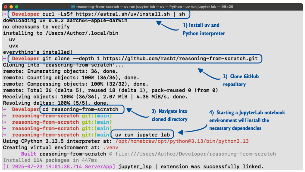
Note that Figure 2.3 steps through the uv installation and usage on a macOS terminal, but uv is supported by Linux and Windows as well.

1. To install uv, run the installation for your OS from the official website: https://docs.astral.sh/uv/getting-started/installation/

2. Next, clone the GitHub repo:

    git clone --depth 1 <https://github.com/rasbt/reasoning-from-scratch.git>
       
   

   Here, the --depth 1 option tells git to perform a shallow clone, which means it only downloads the latest version of the code without the full version history. This makes the download faster and uses less space.

   If you don’t have git installed, you can also manually download the source code repository from the publisher’s website or by opening this link in your browser: https://github.com/rasbt/reasoning-from-scratch/archive/refs/heads/main.zip (unzip it after downloading).

3. Next, in the terminal, navigate to the reasoning-from-scratch folder.

4. Inside the reasoning-from-scratch folder, execute:

    uv run jupyter lab
       
   

The command above will launch JupyterLab, where you can open a blank Jupyter notebook to type and execute code or open the Chapter 2 notebook that contains all the code covered in this chapter.

Tip: Python script files can be executed via uv run script-name.py.

The above uv run... command also sets up a local virtual environment (usually inside an invisible .venv/ folder) and installs all dependencies from the pyproject.toml file inside the reasoning-from-scratch folder automatically. So, the manual installation of code dependencies via the requirements file is not needed. However, if you plan to install additional packages, you can use the following command:

uv add packagename

The supplementary code repository contains additional installation instructions and details inside the ch02 subfolder if needed.

2.3 Understanding hardware needs and recommendations

You may have heard that training LLMs is very expensive. For leading LLM companies, it is not uncommon to spend anywhere between 1-10 million dollars on the small end and >50 million dollars on the high end in terms of compute costs to train a new base model LLM before even adding any reasoning techniques.

For example, the DeepSeek V3 model, which serves as the base checkpoint for the DeepSeek R1 reasoning system, was trained on 2,048 Nvidia H800 GPUs for about 11 weeks with an estimated cost of 5.5 million USD. (DeepSeek V3 is one of the few more recent models with a fully transparent compute disclosure.)

Furthermore, according to the technical report, the final training run used 14.8 million GPU-hours of compute. The energy usage was roughly 620 MWh, which is roughly the amount of electricity that an average American household uses in about 55 years.

This resource requirement and high price tag would make the development of an LLM unfeasible for me and most readers. So, we are going to use a relatively small (but capable) pre-trained LLM on top of which we implement reasoning techniques.

Note that this smaller LLM is a scaled-down version that otherwise follows the same architecture as contemporary state-of-the-art models. And the reasoning methods that we will apply are the same as those used by larger LLMs. The difference is that the smaller LLM allows us to explore these methods in a budget-friendly way.

As an analogy, imagine you are curious to learn how cars work. If you are new to cars, as a learning exercise, you probably wouldn’t start out building an expensive Ferrari right away. Instead, you would, for example, create a smaller car like a Volkswagen Beetle to start with, which still teaches you a lot about how engines and the transmissions work. On the contrary, I would even say that working on a smaller car helps you better understand how the engine and transmissions work because it gets complicated refinements and other details out of the way.

However, while we will use a relatively small model for these educational purposes in this book, the usage, development, and application of the reasoning techniques are still computationally intensive, and later chapters, such as chapters 5-8, will benefit from using a GPU.

If you followed the previous section, you should have PyTorch installed, which you can use to see if your computer has a PyTorch-supported GPU by executing the following PyTorch code in Python:

import torch

print(f"PyTorch version {torch.__version__}")
if torch.cuda.is_available():
    print("CUDA GPU")
elif torch.mps.is_available():
    print("Apple Silicon GPU")
else:
    print("Only CPU")

Depending on your machine, the code may return:

PyTorch version 2.7.1
Only CPU

Don’t worry if your machine does not have a GPU to run the code. Chapters 2-5 can be executed in a reasonable time on a CPU.

Depending on the chapter, the code will automatically use an NVIDIA GPU if available, otherwise run on the CPU (or Apple Silicon GPU if recommended for a particular section or chapter). However, I will provide more information in the respective sections and chapters.

Like many other AI researchers who work on and with LLMs daily, I don’t have a machine with the necessary GPU hardware to train LLMs at home and use cloud resources instead. If you are looking for cloud provider options, my personal preference is Lightning AI Studio (https://lightning.ai/), due to its ease of use and feature support, as shown in Figure 2.4. Alternatively, Google Colab (https://colab.research.google.com/) is another good choice.

Figure 2.4 An overview of the Lightning AI GPU cloud platform in a web browser. The interface supports Python scripts, Jupyter notebooks, terminal access, and lets users switch between CPU and various GPU types based on their compute needs.

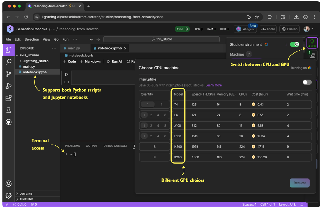
As of this writing, Lightning AI also offers users free compute credits after the sign-up and verification process, which can be used for the different GPU choices shown in Figure 2.4. (As mentioned before, a GPU is not needed for this chapter; however, if you want to use a GPU, the T4 GPU is more than sufficient for this chapter.)

Note: For disclosure, I helped build and launch the Lightning AI platform in 2023 and still hold a small stake. I am not sponsored to recommend it and pay for it myself. I use it because I simply find it the most convenient. It supports multiple types of GPUs, allows easy switching between them and back to CPU to save costs, and lets me pause or resume environments without eroding the setup.

The supplementary code repository contains additional GPU platform recommendations inside the ch02 subfolder if needed.

Using PyTorch

In this section, we imported and used the PyTorch library, which is currently the most widely used general-purpose library. We will use it throughout this book to run and train LLMs, including the reasoning methods we will develop. If you are new to PyTorch, to get the most out of this book, I recommend reading through my PyTorch in One Hour: From Tensors to Training Neural Networks on Multiple GPUs tutorial, which is freely available on my website at https://sebastianraschka.com/teaching/pytorch-1h.

2.4 Preparing input texts for LLMs

In this section, we explore how to use a tokenizer to process input and output text for an LLM, as shown in Figure 2.5, which expands on the input and output preparation steps shown earlier in Figure 2.2 to provide a more detailed view of the tokenization pipeline.

Figure 2.5 A simplified illustration of how an LLM receives input data and generates output. The user-provided text is tokenized into IDs using the tokenizer’s encode method, which are then processed by the LLM to generate output token IDs. These are decoded back into human-readable text using the tokenizer’s decode method.

To see how this works in practice, we will begin by loading a tokenizer from this book’s reasoning-from-scratch Python package, which should have been installed according to the instructions in Section 2.2.

To download the tokenizer files (corresponding to the Qwen3 base LLM, which we will introduce in the next section), run:

from reasoning_from_scratch.qwen3 import download_qwen3_small
download_qwen3_small(kind="base", tokenizer_only=True, out_dir="qwen3")

This will display a progress bar similar to:

tokenizer-base.json: 100% (6 MiB / 6 MiB)

The command downloads the tokenizer-base.json file (approximately 6 megabytes in size) and saves it in a qwen3 subdirectory.

Now, we can load the tokenizer settings from the tokenizer file into the Qwen3Tokenizer:

from pathlib import Path
from reasoning_from_scratch.qwen3 import Qwen3Tokenizer

tokenizer_path = Path("qwen3") / "tokenizer-base.json"
tokenizer = Qwen3Tokenizer(tokenizer_file_path=tokenizer_path)

Since we have not loaded the LLM yet (the central component shown in Figure 2.5), we will first do a simpler dry run using just the tokenizer. Specifically, we will do a tokenization round-trip, that is, we will encode a text into token IDs and then decode those IDs back into text, as illustrated in Figure 2.6.

Figure 2.6 A demonstration of the round-trip tokenization process using a tokenizer. The user-provided input text is first converted into token IDs using the encode method, and then accurately reconstructed back into the original text using the decode method.

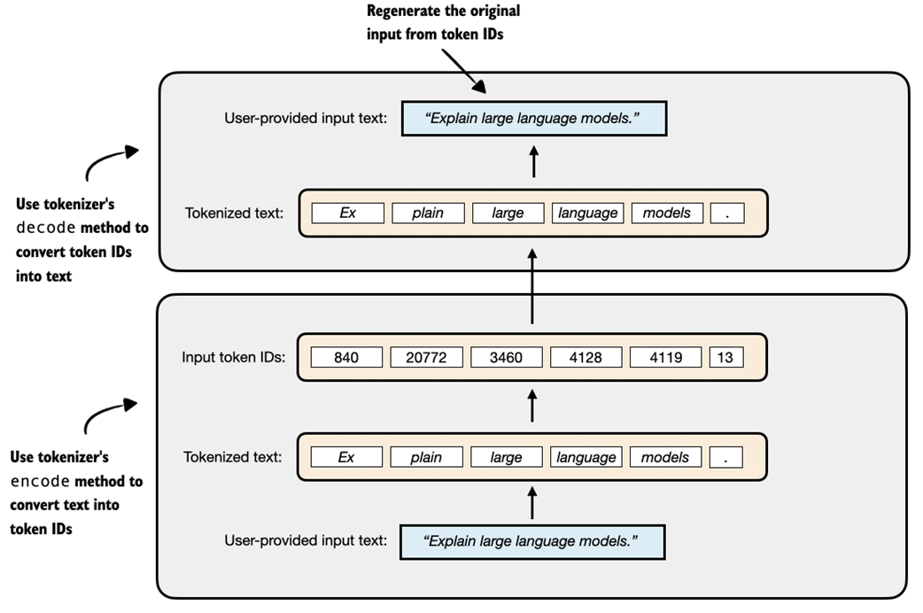
The following code snippet implements the encoding process shown at the bottom of Figure 2.6:

prompt = "Explain large language models."
input_token_ids_list = tokenizer.encode(prompt)

And the following code implements the decoding process, converting the token IDs back into text, shown at the top of Figure 2.6:

text = tokenizer.decode(input_token_ids_list)
print(text)

Based on the printed results, we can see that the tokenizer reconstructed the original input prompt from the token IDs:

'Explain large language models.'

Before we move on to the LLM, let’s take a look at the token IDs that were generated by the encode method. The following code prints each token ID and its corresponding decoded string to help illustrate how the tokenizer works:

for i in input_token_ids_list:
    print(f"{[i]} --> {tokenizer.decode([i])}")

The output is as follows:

840 --> Ex
20772 --> plain
3460 -->  large
4128 -->  language
4119 -->  models
13 --> .

As shown in the output, the original text is split into six token IDs. Each token represents a word or subword, depending on how the tokenizer segments the input.

For example, “Explain” was split into two separate tokens, “Ex” and “plain”. This is because the tokenizer algorithm uses a subword-based method based on Byte Pair Encoding (BPE). BPE can represent both common and rare words using a mix of full words and subword units. Spaces are also often included in tokens (for example, “ large”), which helps the LLM detect word boundaries.

The Qwen3Tokenizer has a vocabulary of about 151,000 tokens, which is considered relatively large as of this writing (for comparison, the early GPT-2 had a vocabulary size of approximately 50,000 tokens, and Llama 3 has a vocabulary size of approximately 128,000 tokens).

A larger vocabulary in a language model increases its size and computational cost for each individually generated token, but it also allows more words to be represented as single tokens rather than being split into subword components. This is beneficial because splitting a word (like breaking “Explain” into “Ex” and “plain”) results in more input tokens. More tokens lead to longer input sequences, which increases processing time and resource usage. For instance, doubling the number of tokens can roughly double the computational cost of running the model as it needs to generate more tokens to complete the response.

Unfortunately, a detailed coverage and from-scratch implementation of a tokenizer is outside the scope of this book. However, interested readers can find additional resources, including my from-scratch implementation, in the further resources and reading sections in Appendix C.

Exercise 2.1: Encoding unknown words

Experiment with the tokenizer to see if and how it handles unknown words. For this, get creative and make up words that don’t exist. Also, if you speak multiple languages, try to encode words in a different language than English.

2.5 Loading pre-trained models

In the previous section, we loaded and familiarized ourselves with the tokenizer that prepares the input data for an LLM and converts LLM outputs back into a human-readable text representation. In this section, we will load the LLM itself, as shown in the overview in Figure 2.7.

Figure 2.7 An overview of the four key stages in developing a reasoning model in this book. This section focuses on loading pre-trained LLM in Stage 1.

As mentioned in the previous section, this book uses Qwen3 0.6B as a base model. In this section, we load its pre-trained weights, as shown in Figure 2.7. The “0.6B” in the model name indicates that the model contains approximately 0.6 billion weight parameters.

Why Qwen3? After carefully evaluating several open-weight base models, I chose Qwen3 0.6B for the following reasons:

• For this book, we want a small but capable open-weight model that can run on consumer hardware.
• The larger variants of the Qwen3 model family are, as of this writing, the leading open-weight models in terms of modeling performance.
• Qwen3 0.6B is more memory-efficient compared to Llama 3 1B and Gemma 2 1B.
• Qwen3 offers both a base model (the focus of our reasoning model development) and an official reasoning variant that we can use as a reference for evaluation purposes.

Note: The canonical spelling of “Qwen3” does not include whitespace, whereas “Llama 3” does.

In line with the spirit of building things “from scratch,” this book uses a custom reimplementation of Qwen3 that I wrote in pure PyTorch, which is entirely independent of external LLM libraries. The emphasis of this reimplementation is on code readability and tweakability, in case you want to modify it later for your own experiments. Despite being built from scratch, this implementation remains fully compatible with the original pre-trained Qwen3 model weights.

However, this book does not cover the Qwen3 code implementation in depth. This topic alone would fill an entire separate book, similar to my other book, Build a Large Language Model (From Scratch). Instead, this Build A Reasoning Model (From Scratch) book specifically focuses on implementing reasoning methods on top of a base model, in this case, Qwen3.

Note: This reimplemented Qwen3 LLM runs entirely locally, just like any other neural network implemented in PyTorch. There are no server-side components or external API calls involved. All model usage happens on your own machine, and your data stays on your device. If you are concerned about privacy, the setup we are using ensures full control over both the LLM inputs and outputs.

For those interested in additional details about Qwen3, as well as the model code, please see Appendix B.

Before we load the model, we can specify the device we are going to use, namely, CPU or GPU. The following code in Listing 2.1 will select the best-available device automatically:

Listing 2.1 Get device automatically

def get_device(enable_tensor_cores=True):
    if torch.cuda.is_available():
        device = torch.device("cuda")
        print("Using NVIDIA CUDA GPU")

        if enable_tensor_cores:
            major, minor = map(int, torch.__version__.split(".")[:2])
            if (major, minor) >= (2, 9):
                torch.backends.cuda.matmul.fp32_precision = "tf32"
                torch.backends.cudnn.conv.fp32_precision = "tf32"
            else:
                torch.backends.cuda.matmul.allow_tf32 = True
                torch.backends.cudnn.allow_tf32 = True

    elif torch.backends.mps.is_available():
        device = torch.device("mps")
        print("Using Apple Silicon GPU (MPS)")

    elif torch.xpu.is_available():
        device = torch.device("xpu")
        print("Using Intel GPU")

    else:
        device = torch.device("cpu")
        print("Using CPU")

    return device

Note that if you have a modern NVIDIA GPU (based on the Ampere architecture or newer), the get_device() function automatically enables Tensor Cores for faster matrix multiplications when enable_tensor_cores=True. This can slightly change floating-point rounding but does not noticeably affect results in this book, and the speed advantage on newer cards is worth it. On non-NVIDIA devices, these settings are ignored.

Using the code from Listing 2.1, we can then obtain the device as follows:

device = get_device()

While GPUs generally provide substantial speed and performance improvements, it can be helpful to initially run the remaining code in this chapter using the CPU for compatibility and debugging purposes. You can temporarily override the automatic selection by explicitly setting:

device = torch.device("cpu")

After finishing the chapter and verifying the code works properly on the CPU, remove or comment out the manual override and rerun the code. If your system has a GPU, you should then observe improved performance.

Note: The code in the remainder of this chapter was executed on a Mac Mini with an Apple M4 CPU. Performance comparisons with the Apple Silicon M4 GPU and the NVIDIA H100 GPU are included at the end of the chapter.

However, before we load the model and put it onto the selected device, we first need to download the weights for Qwen3 0.6B. These files are required to initialize the pre-trained model correctly:

download_qwen3_small(kind="base", tokenizer_only=False, out_dir="qwen3")

The output is as follows:

qwen3-0.6B-base.pth: 100% (1433 MiB / 1433 MiB)
✓ qwen3/tokenizer-base.json already up-to-date

(There is a checkmark in front of the tokenizer because we already downloaded it in the previous section.)

After downloading the model weights via the previous step, we can now instantiate a Qwen3Model class into which we load the pre-trained weights via PyTorch’s load_state_dict method:

from reasoning_from_scratch.qwen3 import Qwen3Model, QWEN_CONFIG_06_B

model_path = Path("qwen3") / "qwen3-0.6B-base.pth"
model = Qwen3Model(QWEN_CONFIG_06_B)
model.load_state_dict(torch.load(model_path))
model.to(device)

Note that if the device setting is "cpu", the model.to(device) operation will be skipped because the model already sits in CPU memory by default.

After executing the code above, you should see the following output (if you are not running the code in an interactive environment like a Jupyter notebook, you have to run print(model) to see the output):

Qwen3Model(
  (tok_emb): Embedding(151936, 1024)
  (trf_blocks): ModuleList(
    (0-27): 28 x TransformerBlock(
      (att): GroupedQueryAttention(
        (W_query): Linear(in_features=1024, out_features=2048, bias=False)
        (W_key): Linear(in_features=1024, out_features=1024, bias=False)
        (W_value): Linear(in_features=1024, out_features=1024, bias=False)
        (out_proj): Linear(in_features=2048, out_features=1024, bias=False)
        (q_norm): RMSNorm()
        (k_norm): RMSNorm()
      )
      (ff): FeedForward(
        (fc1): Linear(in_features=1024, out_features=3072, bias=False)
        (fc2): Linear(in_features=1024, out_features=3072, bias=False)
        (fc3): Linear(in_features=3072, out_features=1024, bias=False)
      )
      (norm1): RMSNorm()
      (norm2): RMSNorm()
    )
  )
  (final_norm): RMSNorm()
  (out_head): Linear(in_features=1024, out_features=151936, bias=False)
)

This output is a summary of the Qwen3 0.6B base model architecture, as printed by PyTorch. It highlights the model’s core components: an embedding layer, a stack of 28 transformer blocks, and a final linear projection head. Each transformer block includes a grouped-query attention mechanism and a multi-layer feedforward network, along with normalization layers throughout.

These components are also illustrated visually in Figure 2.8 for readers familiar with LLM architectures. However, a detailed understanding of this architecture is not required for this book. Since we are not modifying the base model itself, but rather building reasoning methods on top of it, you can safely treat the architecture as a black box for now. However, interested readers can optionally find more information on these components, such as RMSNorm, in Appendix B.

Figure 2.8 Overview of the Qwen3 0.6B model architecture, as instantiated earlier. Input text is tokenized and passed through an embedding layer, followed by 28 repeated transformer blocks. Each block contains grouped-query attention, feedforward layers, and RMS normalization. The model ends with a final normalization and linear output layer. Arrows show the data flow through the model.

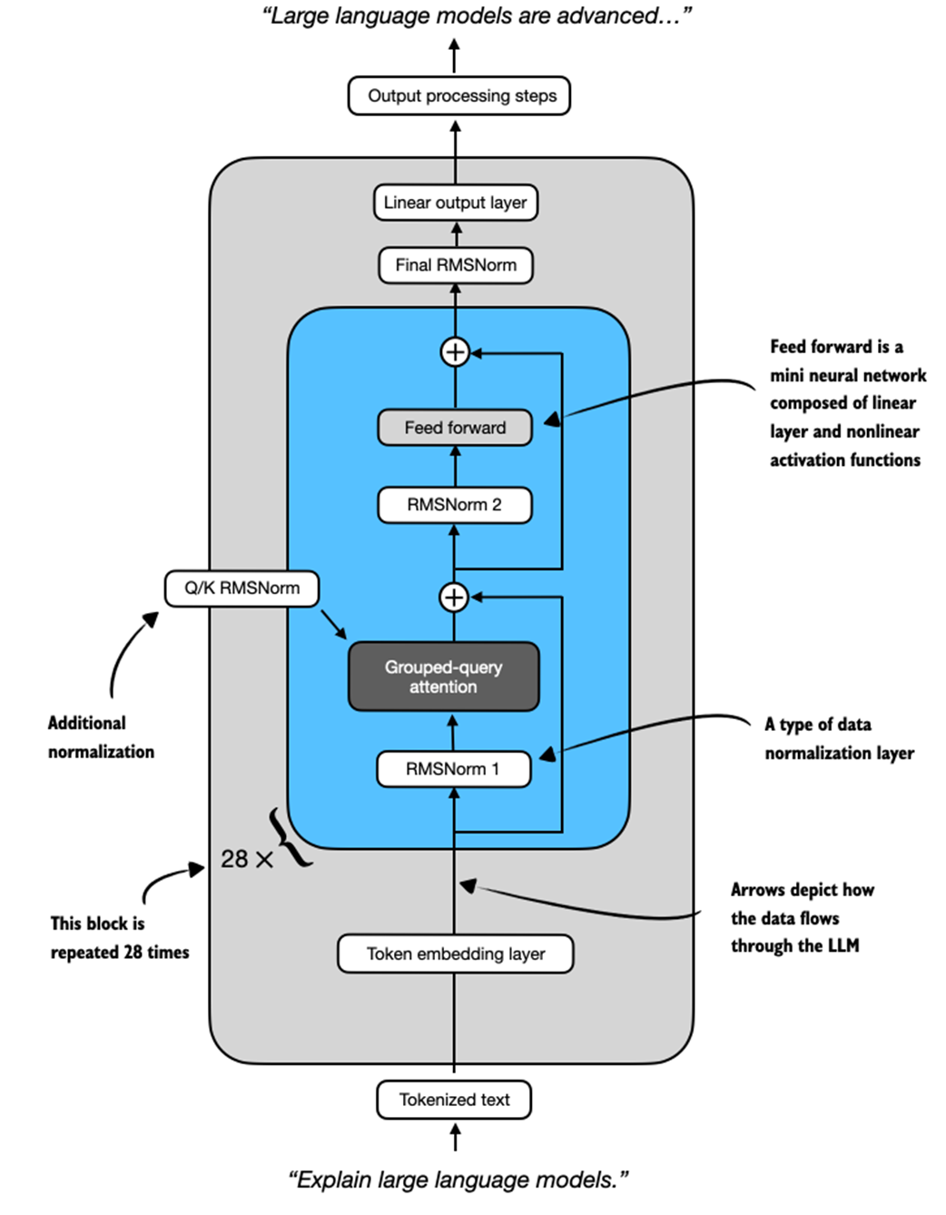
The key takeaway from this section is that we have now loaded a pre-trained model, with its architecture shown in Figure 2.8, that should be capable of generating coherent text. In the next section, we will code a text generation function that feeds tokenized data into the model and returns the response in a human-readable format.

2.6 Understanding the sequential LLM text generation process

After loading a pre-trained LLM, our goal is to write a function that leverages the LLM to generate text. This function forms the foundation for reasoning-improving methods that we will implement later in the book, as shown in Figure 2.9.

Figure 2.9 An overview of the four key stages in developing a reasoning model in this book. This section explains the main concept behind text generation in LLMs, which allows us to implement a text generation function for using the pre-trained LLM in the remainder of this chapter.

However, before we get to implement this text generation function that we will use in this and upcoming chapters (as shown in Figure 2.9), let’s go over the basic concept behind text generation in LLMs.

You may already know that text generation in LLMs is a sequential process where LLMs generate one word at a time. This is often also called autoregressive text generation and is shown in Figure 2.10.

Figure 2.10 An illustration of the sequential (autoregressive) text generation in LLMs. At each iteration, the model generates the next token based on the input and previously generated tokens, which are cumulatively fed back into the model to produce coherent output.

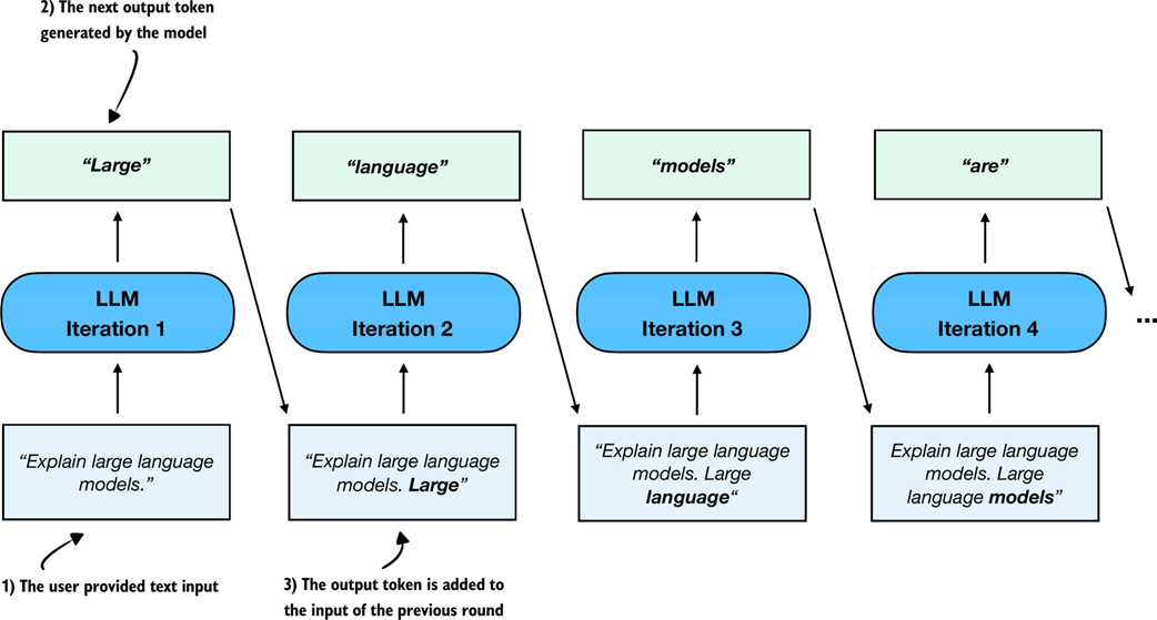
Note that the sequential text generation process shown in Figure 2.10 is a broad overview. The figure shows one generated output token (the box) at each step, when feeding it with an input prompt. This is done for simplicity to explain the main concept behind LLM-based text generation.

Chatbot interfaces

While the diagram in Figure 2.10 shows the underlying next-token prediction process, a chat interface simply wraps this mechanism in a conversational loop. The model still predicts one token at a time, but the system feeds the entire dialogue history back into the model so that each new reply feels context-aware and coherent from turn to turn. This book focuses on single-turn conversations, where the current answer is independent of previous answers. However, interested readers can find an implementation of a chat interface with answer history in Appendix D.

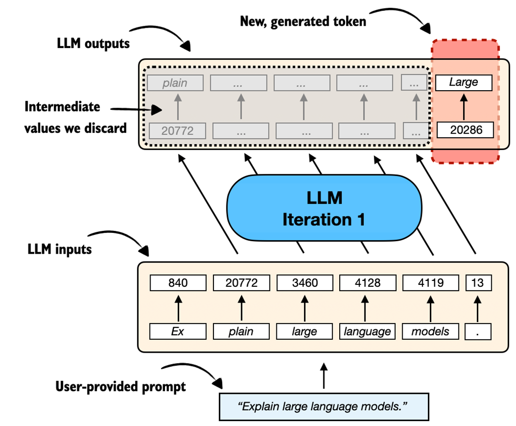
Now, if we look at one of these iterations more closely, an LLM generates one output token for each input token. This means that if we have six input tokens, the LLM returns six output tokens, as illustrated in Figure 2.11. However, it is important to note that we only care about the last generated token in each iteration.

Figure 2.11 A closer look at a single iteration of the autoregressive text generation process. The LLM generates an output sequence that mirrors the input but is shifted one position to the right. At each iteration, the model predicts the next token in the sequence. The LLM effectively learns to continue the input prompt one token at a time.

Before implementing a text-generation function that uses the concept shown in Figure 2.11 for each iteration to implement the autoregressive text generation process shown in Figure 2.10, let’s take a look at a code example to illustrate Figure 2.11 further by reusing the “Explain large language models.” example prompt from Section 2.4:

prompt = "Explain large language models."
input_token_ids_list = tokenizer.encode(prompt)
print(f"Number of input tokens: {len(input_token_ids_list)}")

input_tensor = torch.tensor(input_token_ids_list)
input_tensor_fmt = input_tensor.unsqueeze(0)
input_tensor_fmt = input_tensor_fmt.to(device)

output_tensor = model(input_tensor_fmt)
output_tensor_fmt = output_tensor.squeeze(0)
print(f"Formatted Output tensor shape: {output_tensor_fmt.shape}")

Squeezing and unsqueezing tensors

Tensors are generalized matrices of $n$ dimensions. Many PyTorch functions and model components expect tensors with specific dimensions, so being able to add or remove dimensions is important for making data compatible with these operations.

The .squeeze() and .unsqueeze() operations in PyTorch are used to change the shape of a tensor by removing or adding dimensions of size 1. This is often useful for reshaping a tensor to match what a model expects. For example, a model might expect input tensors with two dimensions (e.g., rows and columns) so it can process batches of inputs (see Appendix F). But if the input is just a row vector, we can use .unsqueeze(0) to add an extra dimension and make it compatible:

example = torch.tensor([1, 2, 3])
print(example)
print(example.unsqueeze(0))

This returns:

tensor([1, 2, 3])
tensor([[1, 2, 3]])

Here, .unsqueeze(0) adds a new dimension at position 0, turning a 1D tensor into a 2D tensor with shape (1, 3). Conversely, .squeeze(0) removes a dimension of size 1 from position 0:

example = torch.tensor([[1, 2, 3]])
print(example)
print(example.squeeze(0))

This returns:

tensor([[1, 2, 3]])
tensor([1, 2, 3])

This is useful when you want to remove extra dimensions that are not needed.

The output from the previous code example is as follows:

Number of input tokens: 6
Formatted Output tensor shape: torch.Size([6, 151936])

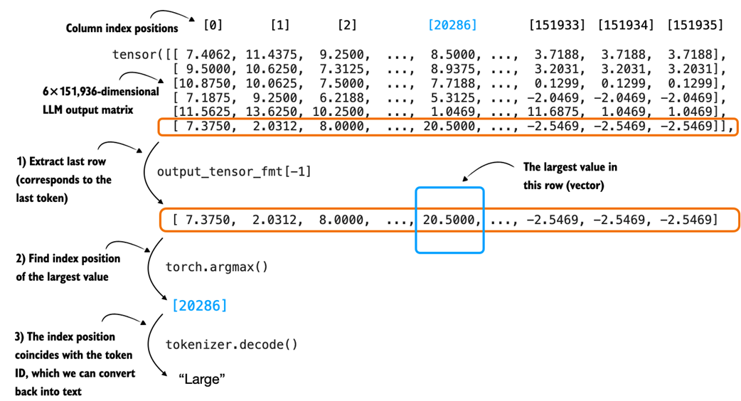
As we can see, we feed six input tokens into the model, which returns a 6×151,936-dimensional matrix. The 6 in this matrix corresponds to the six input tokens. The second dimension, 151,936, corresponds to the vocabulary size that the model supports. For instance, each of the six tokens is represented by a vector with 151,936 values. We can think of the values in these vectors as scores for each possible word in the vocabulary, where the highest score corresponds to the most likely word or subword (in the 151,936-entry vocabulary) to be chosen as the generated token.

So, to get the next generated word, we extract the last row of this 6×151,936-dimensional matrix, find the token ID corresponding to the largest score value in this row, and convert this token ID back into text via the tokenizer, as illustrated in Figure 2.12.

Figure 2.12 A closer look at how the raw scores output by an LLM, in a single text generation iteration, are converted into a token ID and its corresponding text representation.

Let’s see how we can convert the LLM output matrix into the generated text token (shown in Figure 2.12) in code:

Note that LLMs are trained with a next-word prediction task, and as shown in Figure 2.11, we are only interested in the last token, which we can obtain via the [-1] index:

last_token = output_tensor_fmt[-1].detach()
print(last_token)

Here, .detach() separates the tensor from the part of the system that tracks how the model learns. In simple terms, it lets us take the last token from the model’s output and use it for the next step without keeping extra information we don’t need during generation. This saves memory and can make things run faster.

This prints the 151,936 values corresponding to the last token:

tensor([ 7.3750,  2.0312,  8.0000,  ..., -2.5469, -2.5469, -2.5469],
       dtype=torch.bfloat16)

Then, we can use the argmax function to obtain the position with the largest value score (value) in this tensor:

print(last_token.argmax(dim=-1, keepdim=True))

The result is:

tensor([20286])

This returned integer value is the position of the largest value in this vector, and it also corresponds to the token ID of the generated token (last_token), which we can translate back into text via the tokenizer:

print(tokenizer.decode([20286]))

This prints the generated token:

Large

Max versus argmax

It is helpful to briefly recall how max and argmax work and how they differ, since we will use torch.argmax() later when we select the next token when implementing the text generation function.

The torch.max() and torch.argmax() functions in PyTorch are used to find the largest value in a tensor and the index of that value. For example:

example = torch.tensor([-2, 1, 3, 1])
print(torch.max(example))
print(torch.argmax(example))

This returns:

tensor(3)
tensor(2)

The maximum value is 3, and it first appears at index 2.

We can also use keepdim=True with torch.argmax() to keep the output shape consistent by retaining the reduced dimension:

print(torch.argmax(example, keepdim=True))

This returns:

tensor([2])

Here, keepdim=True keeps the result as a 1D tensor with the same number of dimensions as the input, which can be helpful for keeping the shape required by the tokenizer and for concatenation later on in our text generation function.

To recap, Figure 2.10 illustrated the iterative (autoregressive) text generation process in an LLM. Then, Figure 2.11 zooms in on one of the iterations in this process. Figure 2.12 then further zoomed into this one iteration and shows how the score matrix (output by an LLM), gets converted into a token ID (and its corresponding text representation).

While we have seen how to use the LLM to generate a single token, in the next section, we will put these concepts into action and implement a function that applies this concept sequentially to generate coherent output text.

2.7 Coding a minimal text generation function

The previous section explained a single iteration in the basic, sequential text generation process in LLMs. In this section, building on that concept, we will implement a text generation function that uses the pre-trained LLM to generate coherent text following a user prompt, as illustrated in Figure 2.13 in the chapter overview.

Figure 2.13 An overview of the four key stages in developing a reasoning model in this book. In this section we implement a text generation function for the pre-trained LLM.

This text generation function, mentioned in Figure 2.13, works by first converting the input prompt into token IDs that the model can process. The model then predicts the next most likely token, appends it to the sequence, and reprocesses the extended sequence to generate the next token. This iterative process continues until a stopping condition is met, and the generated token IDs are then decoded back into text.

Figure 2.14 shows this process step by step, with both the generated token IDs and their corresponding text at each stage. (This figure is similar to Figure 2.10 shown at the beginning of the previous section, except it shows the generated token IDs alongside their text representation.)

Figure 2.14 An illustration of sequential (autoregressive) text generation in large language models (LLMs), with token IDs shown explicitly. At each iteration, the model generates the next token based on the original input and all previously generated tokens. The predicted token is added to the sequence in both its textual and token ID form.

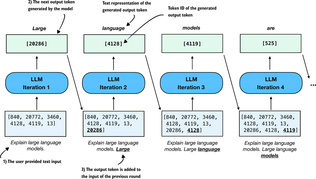
The generate_text_basic function in Listing 2.2 below implements the sequential text generation process (Figure 2.14) using the argmax function introduced in the previous section:

Listing 2.2 A basic text generation function

@torch.inference_mode()
def generate_text_basic(
    model,
    token_ids,
    max_new_tokens,
    eos_token_id=None
):
    input_length = token_ids.shape[1]
    model.eval()

    for _ in range(max_new_tokens):
        out = model(token_ids)[:, -1]
        next_token = torch.argmax(out, dim=-1, keepdim=True)

        if (eos_token_id is not None
                and next_token.item() == eos_token_id):
            break

        token_ids = torch.cat(
            [token_ids, next_token], dim=1)
    return token_ids[:, input_length:]

In essence, the generate_text_basic function in Listing 2.2 applies the argmax-based token ID extraction via a for-loop for a user-specified number of iterations (max_new_tokens). It returns the generated token IDs, similar to what’s shown in Figure 2.14, which we can then convert back into text via the tokenizer.

Let’s use the function to generate a 100-token response to a simple “Explain large language models in a single sentence.” prompt to make sure that the Qwen3Model and generate_text_basic function work (we get to the reasoning task examples in later chapters).

Please note that the following code will be slow and can take 1-3 minutes to complete, depending on your computer (we will speed it up in later sections):

prompt = "Explain large language models in a single sentence."
input_token_ids_tensor = torch.tensor(
    tokenizer.encode(prompt),
    device=device
    ).unsqueeze(0)

max_new_tokens = 100
output_token_ids_tensor = generate_text_basic(
    model=model,
    token_ids=input_token_ids_tensor,
    max_new_tokens=max_new_tokens,
)
output_text = tokenizer.decode(
    output_token_ids_tensor.squeeze(0).tolist()
)
print(output_text)

The generated output text is as follows:

Large language models are artificial intelligence systems that can
understand, generate, and process human language, enabling them to
perform a wide range of tasks, from answering questions to writing
articles, and even creating creative content.<|endoftext|>Human language
is a complex and dynamic system that has evolved over millions of
years to enable effective communication and social interaction. It is
composed of a vast array of symbols, including letters, numbers, and
words, which are used to convey meaning and express thoughts and
ideas. The evolution of language has

Note that the output above was generated on a CPU. Depending on the device (e.g., CPU versus GPU), the exact wording may vary slightly due to differences in floating-point behavior on different hardware.

As we can see based on the output above, the model follows the instruction quite well by producing a single, clear sentence in response to the prompt. However, it continues generating additional, off-topic text after the special token <|endoftext|>. This token is used during training to mark the end of a document and separate different samples.

Tip: The leading whitespace in “ Large” (the first output word) appears because the model continued the text based on the input prompt but we sliced off the original prompt with token_ids[:, input_length:] in the return line in Listing 2.2. If this leading whitespace bothers you, you can remove it via token_ids[:, input_length:].lstrip() or output_text.lstrip().

When using the model for inference (generating text after training), we typically want it to stop as soon as it produces the special token <|endoftext|>. This token is represented by the ID 151643, which we can confirm using:

print(tokenizer.encode("<|endoftext|>"))

For convenience, this token ID is also saved via the tokenizer.eos_token_id attribute. We can pass this ID to the generate_text_basic function to signal when generation should stop:

output_token_ids_tensor = generate_text_basic(
    model=model,
    token_ids=input_token_ids_tensor,
    max_new_tokens=max_new_tokens,
    eos_token_id=tokenizer.eos_token_id
)
output_text = tokenizer.decode(
    output_token_ids_tensor.squeeze(0).tolist()
)
print(output_text)

The output looks like this:

Large language models are artificial intelligence systems that can
understand, generate, and process human language, enabling them to
perform a wide range of tasks, from answering questions to writing
articles, and even creating creative content.

If we compare the response to the previous response, we can see that the text generation stopped once the end-of-sequence token was encountered.

You may have noticed that generating the response is relatively slow and might take several seconds up to multiple minutes, depending on the hardware.

Exercise 2.2: Streaming token generation

Write a modified version of the generate_text_basic function that returns each token as it is generated and prints it, which is also known as streaming token generation.

The goal of this exercise is to understand how to implement token-by-token text generation, a technique often used in real-time applications like chatbots and interactive assistants.

Tip 1: Use yield instead of return to turn the function into a generator.

Tip 2: Then, outside the function, decode each token using a tokenizer and print it as it’s generated (for token in generate_text_basic_stream(...):...) to simulate streaming output.

Before we wrap up and learn how to speed up this function substantially, let’s implement a simple utility function in Listing 2.3 that measures the runtime of the text generation process:

Listing 2.3 Token generation speed and memory usage

def generate_stats(output_token_ids, tokenizer, start_time,
                   end_time, print_tokens=True):
    total_time = end_time - start_time
    print(f"Time: {total_time:.2f} sec")
    print(f"{int(output_token_ids.numel() / total_time)} tokens/sec")

    for name, backend in (("CUDA", getattr(torch, "cuda", None)),
                          ("XPU", getattr(torch, "xpu", None))):
        if backend is not None and backend.is_available():
            max_mem_bytes = backend.max_memory_allocated()
            max_mem_gb = max_mem_bytes / (1024 ** 3)
            print(f"Max {name} memory allocated: {max_mem_gb:.2f} GB")
            backend.reset_peak_memory_stats()

    if print_tokens:
        output_text = tokenizer.decode(output_token_ids.squeeze(0).tolist())
        print(f"\\n{output_text}")

The generate_stats function in Listing 2.3 will calculate the total runtime, given a start and end time stamp, the generation speed in terms of tokens per second (tokens/sec), and the GPU memory used. Note that the GPU memory usage is currently only computed for CUDA-supported GPUs, as PyTorch lacks similar utility functions for CPUs and Apple Silicon GPUs.

To apply the generate_stats function, we obtain a start_time and end_time stamp immediately before and after running the generate_text_basic function via Python’s time module:

import time

start_time = time.time()
output_token_ids_tensor = generate_text_basic(
    model=model,
    token_ids=input_token_ids_tensor,
    max_new_tokens=max_new_tokens,
    eos_token_id=tokenizer.eos_token_id
)
end_time = time.time()
generate_stats(output_token_ids_tensor, tokenizer, start_time, end_time)

The output, on a Mac Mini M4 CPU, is as follows:

Time: 7.94 sec
5 tokens/sec
 Large language models are artificial intelligence systems that can
understand, generate, and process human language, enabling them to
perform a wide range of tasks, from answering questions to writing
articles, and even creating creative content.

At 5 tokens per second, the generation speed is relatively slow. In the next section, we will implement a caching technique that speeds up the generation process 5-6 fold.

Text generation and inference terminology

When reading LLM literature or software documentation, you will often see the term inference used where you might expect text generation. In a neural network context, inference means something very specific, namely, taking a model whose parameters are already learned and fixed, running a forward pass, and producing a prediction (for example, generating the next token). Nothing is being estimated or learned during this stage. In the forward pass, we are simply applying a function.

This is different from inference in statistics, where the goal is to learn unknown information from data. Statistical inference involves estimating parameters, quantifying uncertainty, or testing hypotheses about a population or data-generating process.

Note, that while in large language model contexts, the model is computing the next-token distribution, and people sometimes say the model is “estimating” or “inferring” the next token, this is not estimation in the statistical sense. At this stage, the model is a fixed function and its parameters are already learned.

So when we call the generate_text_basic function, we are not performing statistical inference. We are performing neural network inference, which is just the forward application of a trained model to produce the next-token distribution and select the next generated token from this distribution.

2.8 Faster inference via KV caching

So now that we have a basic text generation function in place, we can turn our attention to what happens when we actually run it in practice. As you may have noticed, the text generation in the previous section can be a bit slow. That slowdown points us to a key concern: performance during inference.

When running inference with LLMs, which in this context means generating text from a prompt, runtime performance (efficiency) quickly becomes important, especially for long sequences. While the code in this book emphasizes clarity over speed, real-world systems often use engineering tricks to make inference more efficient.

In the remaining two sections, we will cover two fundamental techniques, KV caching and model compilation, as shown in the overview in Figure 2.15, to speed up the text generation.

Figure 2.15 An overview of the four key stages in developing a reasoning model in this book. This section builds on pre-trained LLM and the basic text generation function we coded earlier and applies KV caching to speed up execution.

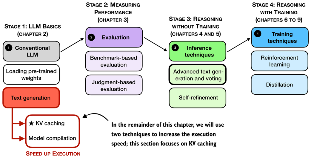
As shown in Figure 2.15, one engineering trick that increases the text generation speed is KV caching, where KV refers to the keys and values used in the model’s attention mechanism. If you are not familiar with these terms, that’s okay. The key idea is that we can cache certain intermediate values and reuse them at each step of text generation, as shown in Figure 2.16, which helps speed up inference.

Figure 2.16 Illustration of how a KV cache improves efficiency during autoregressive text generation. Instead of reprocessing the entire input sequence at each step, the KV cache stores intermediate representations so that the LLM can reuse them to generate the next token. This eliminates the need to concatenate the generated token with prior inputs in each subsequent iteration.

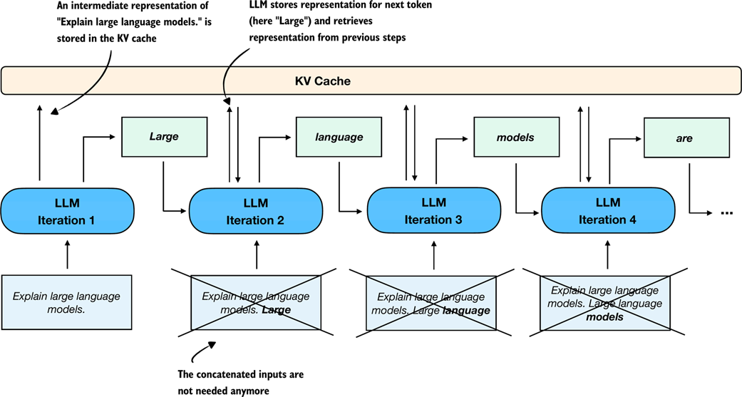
The key idea of KV caching, as shown in Figure 2.16, is to store intermediate values computed in each iteration in a cache. Previously, each new token generated by the network was concatenated to the entire input sequence and fed back into the model repeatedly (indicated by crossed-out boxes in the diagram). This approach was inefficient because all tokens, except the newly generated one, remain identical in subsequent iterations. By using a KV cache, we avoid redundant computation and instead directly retrieve stored intermediate representations.

As mentioned earlier, the non-reasoning focused LLM details like KV caching, which we used to improve the token generation speed, are outside the scope of this book, and they are not required for the topics covered later in this book. However, interested readers can find more information on the mechanics of KV caching in my freely available article: Understanding and Coding the KV Cache in LLMs from Scratch (https://magazine.sebastianraschka.com/p/coding-the-kv-cache-in-llms).

Below is a modified version of the generate_text_basic function that incorporates a KV cache, which is almost identical to the basic text generation function in Listing 2.2, except for the KV cache-related change highlighted via the comments:

Listing 2.4 A basic text generation function with KV cache

from reasoning_from_scratch.qwen3 import KVCache

@torch.inference_mode()
def generate_text_basic_cache(
    model,
    token_ids,
    max_new_tokens,
    eos_token_id=None
):

    input_length = token_ids.shape[1]
    model.eval()
    cache = KVCache(n_layers=model.cfg["n_layers"])
    model.reset_kv_cache()
    out = model(token_ids, cache=cache)[:, -1]

    for _ in range(max_new_tokens):
        next_token = torch.argmax(out, dim=-1, keepdim=True)

        if (eos_token_id is not None
                and next_token.item() == eos_token_id):
            break

        token_ids = torch.cat([token_ids, next_token], dim=1)
        out = model(next_token, cache=cache)[:, -1]

    return token_ids[:, input_length:]

The generate_text_basic_cache function in Listing 2.4 differs only slightly from the generate_text_basic function in Listing 2.2. The main difference is the introduction of a KVCache object.

During the first iteration, the model is given the full input token sequence as before, using model(token_ids, cache=cache). Behind the scenes, the KV cache stores intermediate values for all these input tokens.

In the following iterations, we no longer need to pass the entire sequence. Instead, we only provide the next_token to the model using model(next_token, cache=cache). The model then retrieves the necessary context from the previously stored KV cache.

Let’s time this function to see whether it provides any performance benefits:

start_time = time.time()
output_token_ids_tensor = generate_text_basic_cache(
    model=model,
    token_ids=input_token_ids_tensor,
    max_new_tokens=max_new_tokens,
    eos_token_id=tokenizer.eos_token_id,
)
end_time = time.time()
generate_stats(output_token_ids_tensor, tokenizer, start_time, end_time)

The output is:

Time: 1.40 sec
29 tokens/sec

 Large language models are artificial intelligence systems that can
understand, generate, and process human language, enabling them to
perform a wide range of tasks, from answering questions to writing
articles, and even creating creative content.

As we can see, this approach is significantly faster, generating 29 tokens per second compared to just 5 tokens per second previously (measured on a Mac Mini M4 CPU).

Importantly, we also see that the generated text is the same as before, which is an important sanity check to ensure that the KV cache is implemented and used correctly.

In the next section, we will learn about another technique we can use to further improve the generation speed, which will come in handy when we evaluate the model in the upcoming chapters. Faster generation allows us to run more evaluations in less time and makes it easier to compare different models or settings efficiently.

2.9 Faster inference via PyTorch model compilation

In the previous section, we covered KV caching as a technique to improve runtime efficiency as shown in the overview in Figure 2.17.

Figure 2.17 An overview of the four key stages in developing a reasoning model in this book. This section builds on pre-trained LLM and the basic text generation function we coded earlier, including KV caching, and adds model compilation to speed up the execution speed even further.

As shown in Figure 2.17, in this remaining section of this chapter, we will apply another technique that can substantially speed up model inference: model compilation using torch.compile. This feature allows the model to be compiled ahead of time, which reduces overhead and improves runtime performance during text generation.

major, minor = map(int, torch.__version__.split(".")[:2])
if (major, minor) >= (2, 8):
    # This avoids retriggering model recompilations
    # in PyTorch 2.8 and newer
    # if the model contains code like self.pos = self.pos + 1
    torch._dynamo.config.allow_unspec_int_on_nn_module = True

model_compiled = torch.compile(model)

If you are using a Mac with Apple Silicon and encounter an InductorError, please make sure to use PyTorch 2.9 or newer.

It is worth noting that the first execution using the compiled model may be slower than usual due to the initial compilation and optimization steps. To better measure the performance improvement, we will repeat the text generation process multiple times.

To begin, we will test this using the non-cached version of the generation function. The code in Listing 2.5 is similar to what we used before except that we run it three times in a row. The code execution may take a few minutes to finish, depending on the system:

Listing 2.5 Generating text with the compiled model

for i in range(3):
    start_time = time.time()
    output_token_ids_tensor = generate_text_basic(
        model=model_compiled,
        token_ids=input_token_ids_tensor,
        max_new_tokens=max_new_tokens,
        eos_token_id=tokenizer.eos_token_id
    )
    end_time = time.time()

    if i == 0:
        print("Warm-up run")
    else:
        print(f"Timed run {i}:")
    generate_stats(output_token_ids_tensor, tokenizer, start_time, end_time)

    print(f"\\n{30*'-'}\\n")

The output is as follows:

Warm-up run
Time: 11.68 sec
3 tokens/sec

 Large language models are artificial intelligence systems that can
understand, generate, and process human language, enabling them to
perform a wide range of tasks, from answering questions to writing
articles, and even creating creative content.

------------------------------

Timed run 1:
Time: 6.78 sec
6 tokens/sec
Output text:

 Large language models are artificial intelligence systems that can
understand, generate, and process human language, enabling them to
perform a wide range of tasks, from answering questions to writing
articles, and even creating creative content.

------------------------------

Timed run 2:
Time: 6.80 sec
6 tokens/sec
Output text:

 Large language models are artificial intelligence systems that can
understand, generate, and process human language, enabling them to
perform a wide range of tasks, from answering questions to writing
articles, and even creating creative content.

------------------------------

As we can see from the results above, the compiled model achieves a slight improvement in speed, with around 6 tokens per second compared to the previous 5 tokens per second.

Next, let’s see how the KV cache version performs in comparison, using the same code as before except for swapping generate_text_basic with generate_text_basic_cache:

Listing 2.6 Generating text with the compiled model using a KV cache

for i in range(3):
    start_time = time.time()
    output_token_ids_tensor = generate_text_basic_cache(
        model=model_compiled,
        token_ids=input_token_ids_tensor,
        max_new_tokens=max_new_tokens,
        eos_token_id=tokenizer.eos_token_id
    )
    end_time = time.time()

    if i == 0:
        print("Warm-up run")
        generate_stats(
        output_token_ids_tensor, tokenizer, start_time, end_time
    )
    else:
        print(f"Timed run {i}:")
        generate_stats(output_token_ids, tokenizer, start_time, end_time)

    print(f"\\n{30*'-'}\\n")

The output is as follows:

Warm-up run
Time: 8.07 sec
5 tokens/sec

 Large language models are artificial intelligence systems that can
understand, generate, and process human language, enabling them to
perform a wide range of tasks, from answering questions to writing
articles, and even creating creative content.

------------------------------

Timed run 1:
Time: 0.60 sec
68 tokens/sec
Output text:

 Large language models are artificial intelligence systems that can
understand, generate, and process human language, enabling them to
perform a wide range of tasks, from answering questions to writing
articles, and even creating creative content.

------------------------------

Timed run 2:
Time: 0.60 sec
68 tokens/sec
Output text:

 Large language models are artificial intelligence systems that can
understand, generate, and process human language, enabling them to
perform a wide range of tasks, from answering questions to writing
articles, and even creating creative content.

------------------------------

As we can see based on the outputs above, the model generation speed improved from 29 tokens per second for the uncompiled model with KV cache to 68 tokens per second when the same model is compiled (on a Mac Mini M4 CPU), which is more than a 2-fold speed-up.

If you don’t see any improvement, try running torch.compile with the "max-autotune" mode instead of the default settings. For instance, replace:

model = torch.compile(model)

With:

model = torch.compile(model, mode="max-autotune")

Exercise 2.3: Rerun code on non-CPU devices

If you have access to a GPU, rerun the code in this chapter on a GPU device and compare the runtimes to the CPU runtimes.

In case you are curious how the different model configurations compare on an Apple Silicon GPU and a high-end NVIDIA GPU, see Table 2.1.

Table 2.1 Token generation speeds and GPU memory usage for different model configurations on different hardware

Mode	Hardware	Tokens/sec	GPU memory
Regular	Mac Mini M4 CPU	5	-
Regular compiled	Mac Mini M4 CPU	6	-
KV cache	Mac Mini M4 CPU	28	-
KV cache compiled	Mac Mini M4 CPU	68	-
Regular	Mac Mini M4 GPU	27	-
Regular compiled	Mac Mini M4 GPU	43	-
KV cache	Mac Mini M4 GPU	41	-
KV cache compiled	Mac Mini M4 GPU	71	-
Regular	NVIDIA H100 GPU	51	1.55 GB
Regular compiled	NVIDIA H100 GPU	164	1.81 GB
KV cache	NVIDIA H100 GPU	48	1.52 GB
KV cache compiled	NVIDIA H100 GPU	141	1.81 GB

As shown in the table above, the NVIDIA GPU delivers the best performance, which is expected. The CPU still performs surprisingly well once a KV cache and a compiled model are enabled. However, there are a few important details that explain why the GPU gains are not larger for this particular setup.

First, the model in this chapter is not optimized for GPUs. The implementation aims for a good balance between memory usage and compute speed because memory is the main bottleneck for most readers. A GPU-optimized variant would pre-allocate the full K and V tensors up to the maximum context length (in this case, 40 thousand tokens). This pre-allocation avoids repeated concatenation via torch.cat, but it also increases memory consumption.

With a large context size, pre-allocating, for example, 40 thousand entries for both K and V adds a noticeable footprint. Another approach would be to let users specify a fixed context size at construction time, but that introduces extra configuration overhead. The KV cache used here grows on demand via torch.cat, which is simpler and more memory friendly, although concatenating non-preallocated tensors is a bit slower on GPUs.

I included a GPU-optimized version in the bonus materials, where the KV cache variant is slightly faster than the regular version, but it uses more memory (see https://github.com/rasbt/reasoning-from-scratch/tree/main/ch02/03_optimized-LLM).

Second, the model used for benchmarking is small. Larger models benefit much more from KV caching and from GPU-optimized memory layouts. The same holds for batched inference, where GPUs can better saturate their compute units. With a larger model or a GPU-focused implementation, the performance gap in favor of the NVIDIA GPU would be more pronounced.

All examples were run using a single prompt (i.e., a batch size of 1). For readers interested in how performance scales with multiple inputs, batched inference is discussed in Appendix F.

2.10 Summary

• Using LLMs to generate text involves multiple key steps:
  • Setting up the coding environment to run LLM code and install necessary dependencies.
  • Loading a pre-trained base LLM (such as Qwen3 0.6B), which will be extended with reasoning capabilities in later chapters.
  • Initializing and using a tokenizer, which converts text input into token IDs and decodes output back to human-readable form.
• Text generation in LLMs follows a sequential (autoregressive) process, where the model generates one token at a time by predicting the next most likely token.
• The speed and efficiency of text generation can be improved through:
  • KV caching, which stores intermediate states to avoid recomputing previously encountered input tokens at each step.
  • Model compilation using torch.compile, which optimizes runtime performance.
• This chapter lays the technical foundation for reasoning capabilities in upcoming chapters by implementing a functional, efficient text generation pipeline using a pre-trained base LLM.