Deepseek-V4 and before — getting the foundations right & beyond basics

Understanding the components that drives it: A Practical Guide to mHC, CSA, HCA, and Muon

MITB For All · Follow publication
30 min read · May 9, 2026
James Koh, PhD

This post is made for my students of CS610 of the Apr 2026 term.

Contents

• Background
• Why DeepSeek?
• References
• 1. Fundamentals you should not skip
     • 1.1 Byte Pair Encoding
     • 1.2 Embeddings
     • 1.3 Considering context
     • 1.4 Positional Encodings
     • 1.5 Getting outputs
• 1. Building blocks
     • 2.1 Attention
     • 2.2 Multi-heads Latent Attention (MLA)
     • 2.3 Mixture-of-Experts (MoE)
     • 2.4 Multi-Token Prediction (MTP)
• 1. New stuff in DeepSeek-v4: beyond basics
     • 3.1 Manifold-Constrained Hyper-Connections (mHC)
     • 3.1.1 Hyper-Connections (HC)
     • 3.1.2 Manifold-Constrained Hyper-Connections (mHC)
     • 3.1.3 mHC in DeepSeek-v4
       • 3.2 Compressed Sparse Attention (CSA)
     • 3.2.1 DeepSeek Sparse Attention (DSA)
     • 3.2.2 CSA in DeepSeek-v4
       • 3.3 Heavily Compressed Attention (HCA)
       • 3.4 Muon optimizer
       • 3.5 Infrastructures and Post-Training
• Conclusion

Background

The release of Deepseek-R1 in Jan 2025, with open release of distilled “32B & 70B models on par with OpenAI-o1-mini”, accompanied a plunge in the stock prices of big AI names the following week. Within weeks, I immediately updated the CS610 course contents to teach students from Jan’25 and Apr’25 cohorts about Deploying Deepseek locally.

This year, as I prepare for delivering CS610 for the Apr’26 term, Deepseek released its V4 in Apr 2026, showing performance comparable to Claude-Opus-4.6, GPT-5.4 and Gemini-3.1.

Figure from https://api-docs.deepseek.com/news/news260424

It is good to have a good technical understanding of what’s going on under the hood. Being able to talk about this accurately in internship/job interviews will certainly put you ahead.

Fortunately (or unfortunately, for those with weak foundations), each new release is built upon plenty of foundational knowledge, which means that simply reading the latest paper is nowhere near enough for those new to the party, while referring to citations after citations would lead you down a rabbit hole. That is on top of the fact that V3 and V4 papers combined have over 100 pages in total.

Why DeepSeek?

I choose to focus on the Deepseek family because their accompanying papers provide in-depth detail on the model architecture as well as training process, unlike other closed-source alternatives.

There are many overlaps between v3, r1 and v4, such as Multi-Head Latent Attention and Mixture-of-Experts. All of them also implement Group Relative Policy Optimization (GRPO), which I explain in my Reinforcement Learning course.

Let’s build things step by step. I bet that even 5 years later, these knowledge would still remain relevant as a fundamental building block.

References

For completeness and to provide quick access with a timeline overview, here is a list of relevant papers by DeepSeek and others.

By DeepSeek

• DeepSeek-MoE by Dai et al. (2024) Towards Ultimate Expert Specialization in Mixture-of-Experts Language Models. https://arxiv.org/pdf/2401.06066
• DeepSeek-v3 by Liu et al. (2024) DeepSeek-V3 Technical Report. https://arxiv.org/abs/2412.19437
• DeepSeek-r1 by Guo et al. (2025) DeepSeek-R1: Incentivizing Reasoning Capability in LLMs via Reinforcement Learning. https://arxiv.org/pdf/2501.12948
• DeepSeek-V3.2 (2025) Pushing the Frontier of Open Large Language Models https://arxiv.org/pdf/2512.02556
• DeepSeek-v4 by Deepseek (2026) DeekSeek-V4: Towards Highly Efficient Million-Token Context Intelligence https://huggingface.co/deepseek-ai/DeepSeek-V4-Pro/blob/main/DeepSeek_V4.pdf
• mHC: Manifold-Constrained Hyper-Connections by Xie et al. (2026) https://arxiv.org/pdf/2512.24880

Others

• Attention Is All You Need by Vaswani et al. (2017) https://arxiv.org/abs/1706.03762
• GPT-2 by Radford et al. (2019) Language Models are Unsupervised Multitask Learners. https://cdn.openai.com/better-language-models/language_models_are_unsupervised_multitask_learners.pdf
• GPT-3 by Brown et al. (2020) Language Models are Few-Shot Learners. https://arxiv.org/abs/2005.14165
• GPT-4 by Achiam et al. (2023) GPT-4 Technical Report https://arxiv.org/pdf/2303.08774
• RoFormer by Su et al. (2021/2024) https://arxiv.org/abs/2104.09864v5; https://doi.org/10.1016/j.neucom.2023.127063
• Multi-token Prediction by Gloeckle et al. (2024) https://arxiv.org/pdf/2404.19737
• Hyper Connections by Zhu et al. (ByteDance) (2025) https://openreview.net/pdf?id=9FqARW7dwB

1. Fundamentals you should not skip

I always believe in understanding how inputs are converted into the model’s outputs. Let’s start from the beginning.

DeepSeek, or any LLM for that matter, takes in a string (ie. sequence of characters).

1.1 Byte Pair Encoding

From the input sequence, we first need to decide on the tokens, before it is possible to map to the corresponding vector.

Byte Pair Encoding (BPE) is a sub-word level tokenization approach. It is a middle ground between tokenizing single characters (which does not convey much meaning by themselves) and indiscriminately taking entire words (which loses generalizability).

Although dating back to the 1990’s (Shibata et al. 1999), it is still used in the state-of-the-art models in the 2020’s, both in GPT and DeepSeek. BPE works by iteratively merging the most frequent adjacent pairs of symbols (which starts off as individual characters). Commonly used words would typically simply end up as a single token. The tokenizer for DeepSeek-v3 has a vocabulary of 128,000 tokens (see section 4.1 of DeepSeek-v3).

To illustrate, consider the sentence ‘My father works in a financial corporation.’

import torch
from transformers import AutoTokenizer, AutoModel

tokenizer = AutoTokenizer.from_pretrained(
    "deepseek-ai/deepseek-llm-7b-base"
)
sentence = "My father works in a financial corporation."

tokens = tokenizer.tokenize(sentence, return_tensors="pt")
token_ids = tokenizer(sentence)["input_ids"]
print("Tokens:", tokens)
print("Token IDs:", token_ids)

It becomes the following eight tokens. Notice that the words ‘in’ and ‘a’ are represented with a single token (index 1695), while ‘corporation’ is represented with two tokens.

Tokens: ['My', 'father', 'works', 'ina', 'financial', 'corpor', 'ation', '.']
Token IDs: [3673, 13446, 5774, 1695, 75293, 39656, 335, 13]

The token indices can in turn be used to retrieve the original sub-words.

for idx in token_ids:
    print(tokenizer.decode(idx))

1.2 Embeddings

Having obtained tokens from BPE, we need to represent it mathematically. An embedding can be loosely thought of as a description/representation of a token — eg. whether it is a verb or noun, semantic properties, the connotations it carries, typical associations etc. These values are all learnt (based on their natural occurrences in large corpuses), and might not even be individually interpretable. It is analogous to the feature vector of an image.

There are many classical approaches for how the embeddings $v_i$ are obtained in the very first place, for example using Word2Vec, GloVe, or more fanciful approach like FastText by FAIR.

We can obtain the embeddings by passing a torch tensor into .embed_tokens. The output is a torch.Tensor of shape [1, n_tokens, 4096], where 4096 corresponds to the number of dimensions of the embeddings space.

model = AutoModel.from_pretrained(
    "deepseek-ai/deepseek-llm-7b-base", output_hidden_states=True
)
model.eval()

token_ids = tokenizer(sentence, return_tensors="pt")["input_ids"]
with torch.no_grad():
    token_embeddings = model.embed_tokens(token_ids)

I am using a simple distilled ‘7B’ variant here, rather than using the latest Deepseek-V4, so that any reader can quickly and easily replicate. The concept remains exactly the same.

Screenshot from author showing the composition of model from “deepseek-ai/deepseek-llm-7b-base”.

To get a better feel of things, let’s visualize each token alongside the first four values of their embeddings (of course, we could use PCA or some dimensionality reduction technique, but let’s keep things simple).

token_embeddings[0, :, :4]

tensor([[-3.6621e-02, -1.0010e-01,  3.4375e-01,  3.0469e-01],
        [ 5.1025e-02,  4.7119e-02,  1.8555e-01, -1.2695e-01],
        [ 8.5449e-02,  1.1621e-01,  2.0312e-01,  4.2236e-02],
        [ 4.1992e-02,  8.6914e-02,  3.7500e-01, -9.2773e-03],
        [ 6.0059e-02,  3.3447e-02,  7.8613e-02,  1.5723e-01],
        [-1.7090e-02,  1.0156e-01, -3.3112e-03,  1.7871e-01],
        [ 9.2773e-02, -5.1758e-02,  2.1973e-01,  3.9062e-02],
        [-4.1260e-02, -2.4986e-04,  3.8281e-01, -1.0620e-02]],
       dtype=torch.bfloat16)

Notice that the values are mostly in the order of 0.01 ~ 0.1.

First four embedding values for each token.

Now, if we were to compare the cosine similarity between the token embeddings (dim 4096) of ‘works’ and ‘corpor’, without context, the result is a mere 0.04. This is because the raw token embeddings, in itself, does not capture any sentence semantics. There is no context, nor even knowledge of their relative position in the sentence.

emb_1 = token_embeddings[:,2,:] # for token 'works'
emb_2 = token_embeddings[:,5,:] # for token 'corpor'

from torch.nn.functional import cosine_similarity
cosine_similarity(emb_1, emb_2)

Jumping ahead, if you were to compare the embeddings of the last hidden state, the cosine similarity would increase to 0.707. We shall continue, to see how this is possible.

inputs = tokenizer(sentence, return_tensors="pt")
with torch.no_grad():
    last_hidden_state = model(**inputs).last_hidden_state

state_1 = last_hidden_state[:,2,:] # for token 'works'
state_2 = last_hidden_state[:,5,:] # for token 'corpor'
cosine_similarity(state_1, state_2)

tensor([0.7070], dtype=torch.bfloat16)

Screenshot from author.

1.3 Considering context

Next, consider the phrase “father works at a bank”. Each word/token has their own vector. However, bank could have multiple meanings (financial institution, river bank etc.), and the context depends on other words in the sentence. Therefore, we want a modified vector that is not just word-specific, but also contains context from its neighbours.

Idea of how embedding vectors v1 to v5 can be modified to y1 to y5. We want to incorporate aspects of v2 (‘works’) with v5 (‘bank’), so that the resulting y5 captures information of bank referring to some financial institution. Image by author.

There will not be any ‘single-best-choice’ of W to transform $v_i$ to $y_i$, because it depends on the other tokens. Therefore, it is clearly beneficial to multiply with a learnable matrix, such that the resulting $y_i$ accounts for context.

Considering overall sentence context when transforming $v_i$ to $y_i$, rather than attempting to use one-size-fits-all weights. Image by author.

Note that $q_i$ and $k_i$ and $v_i$ would be different even for the same words, as those would be mapped using different projection matrices (not shown in the figure above):

Q, K, V are the query, key and value representations of all tokens (think words), obtained by projecting the input embeddings X using the learned matrices WQ, WK and WV.

For those who are unclear about linear algebra, the following would be helpful.

Suppose that each x is a vector of length 100, and v is a vector of length 200. The matrix X comprises x1 to x5 (assuming 5 tokens). Shape of V = $XW_{V}$ would be (N, 200) = (N, 100) x (100, 200). In reality, $W_{V}$ is typically square matrices as dimensions are the same; though I used different dimensions to emphasize the math. Note that $W_{V}$ here is very different from W11 to W55 at the beginning of the section; those W11 to W55 themselves could be functions of Q and K.

1.4 Positional Encodings

The attention block does not distinguish between token order. However, the position matters and ought to be taken into account (‘not completely’ and ‘completely not’ hold different meanings).

We’ll start with Sinusoidal Positional Encodings. It is easy to build upon that knowledge to understand Rotary Positional Encodings thereafter. In the Attention paper by Vaswani et al. (2017), the following is given:

Equation from section 3.5 of the ‘Attention Is All You Need’ paper.

Each token position pos is assigned a deterministic vector of length d_{model}. The index i refers to the dimension inside the embedding vector, not the position of a token in the sentence. For a 4096-dimensional space, we have 2048 pairs of (2i, 2i+1).

The gif below shows how the sine component of positional embeddings (PE) vary with respect to token position pos. Each snapshot represents 2048 values of the positional embedding, corresponding to a particular pos; when added to the other 2048 cosine values, we see that each 4096-dimensional pos has its own unique ‘signature’.

Gif by author, created by applying the above PE formula and using matplotlib. Lower-index dimensions change quickly with position, while higher-index dimensions change at a lower frequency. The cosine component follows a similar trend.

This PE vector would be added (superimposed) to the token embeddings, causing information to be ‘blended’, but concatenating the position embedding is not desirable as it leads to a more parameters and training overhead. To illustrate the effects of superposition, I’ve super-imposed two photographs taken by me (one is a plate of food, another is a place).

Superimposed image by author. Imagine that the pixels from the food picture correspond to token embeddings, while pixels from the place picture correspond to positional embeddings.

Positional information can be incorporated in a less ‘invasive’ manner, via rotary positional encoding (RoPE). Here, the d-dimensional embedding space is divided into d/2 subspaces, and vectors are rotated by angles determined according to token position $m$ (called pos above) and $\theta_i$ (formula below).

Screenshot of equation 34 from section 3.4.2 of RoFormer https://arxiv.org/pdf/2104.09864, which is an efficient form of equations 14 and 15 from its section 3.2.2.

Angle $\theta$ is a function of i (dimension inside the embedding vector) and d. Equation from section 3.2.2 of RoFormer.

This is built upon via the use of YaRN (Yet another RoPE extension) for dealing with larger context, as stated in Section 4.3 of the 2024 DeepSeek-V3 paper, citing an earlier 2023 work.

1.5 Getting outputs

When we pass a text input to an LLM and receive an answer, we are actually getting sequential predictions of tokens, pieced together. Each output is incrementally appended to the input sequence, from which the next output token is then predicted.

Outputs are appended as input in generating the subsequent predictions. Since we’re establishing the foundational knowledge, let’s ignore improvements such as Multi-Token Prediction.

It may appear like there would be numerous repeated computations, but the key-value cache lets the model reuse previously computed K and V vectors, so at each generation step it only needs to process the newest token through the Transformer layers while attending to cached past tokens.

2. Building blocks

In DeepSeek-V3, the authors stated that there are 61 Transformer layers, where each layer (block) comprises RMSNorm, multi-head latent attention (section 2.2 of this article), mixture of experts (section 2.3 of this article) and skip connections. You likely already know RMSNorm and skip connections.

Screenshot from Figure 2 of Deepseek-v3 (2024) https://arxiv.org/pdf/2501.12948. Architecture of DeepSeek-V3.

2.1 Attention

Before attention, encoder-decoder sequence models had to compress inputs into a fixed-size context vector, resulting in information bottleneck and hence compromising on the performance especially when dealing with large context.

Notice that in section 1.3 of this article, we were trying to get $y_i$ to account for context (although it is very short, just for illustration). This is achievable in the attention mechanism.

Screenshot from Figure 2 of ‘Attention Is All You Need’ https://arxiv.org/pdf/1706.03762. We will focus on the left side (just attention) first, and look at multi-head attention in a later subsection.

You would have seen the above image in many places. Let’s ensure we know why and how the mathematical operations are performed here.

Mathematically, the left diagram above is simply describing the following equation.

Equation (1) in section 3.2.1 of the Attention paper https://arxiv.org/pdf/1706.03762.

The flowchart showing the intermediate steps might make the process clearer to you.

Image by author

In self-attention, the same X (which may be input embeddings, if we are in the first layer, or some intermediate hidden state) is used to obtain Q, K, and V, while in cross-attention, Q comes from one sequence while K and V comes from another.

The Deepseek variants, whose architectures are disclosed and can be verified, are actually decoder-only LLMs, hence we will focus on self-attention. The attention matrix is causally masked, i.e. each token may attend only to itself and to earlier tokens, but not to future tokens.

For n tokens, the attention matrix will be of shape (n, n), where each component of the attention matrix $a_{i,j}$ denotes how much token i attends to token j.

2.2 Multi-heads Latent Attention (MLA)

We move on to the rationale for ‘multi-headed’ attention. A sentence usually contains several relationships that must be interpreted simultaneously. Think of a sentence, say “My father works at a bank where overtime is discouraged”.

A single attention head can already let each token attend to every other token, but it can capture only one pattern. With multi-heads, one head may focus on the relationships like ‘My’ and ‘father’ (not ‘My’ and ‘bank’), another may associate locations like ‘works’ with ‘bank’, while a third may track sentiments like ‘overtime’ and ‘discouraged’.

It would not be that straightforward and well-partitioned, of course, and we’ll just leave it to the model to learn whatever works best during training.

As stated in Section 4.2 of the DeepSeek-V3 paper, the number of attention heads is 128, and the per-head dimension is also 128.

We now look at the ‘latent’ in MLA.

The idea of storing KV (key value) cache is to avoid repeated computations, as alluded to in section 1.5 above. However, this causes another issue. If we store everything, the cache is very large, which gets expensive for long context.

\(\mathbf{c}_t^{KV} = W^{DKV}\mathbf{h}_t, \quad \text{where } \mathbf{c}_t^{KV} \in \mathbb{R}^{d_c} \text{ and } d_c \ll d_hn_h\) \([\mathbf{k}_{t,1}^C; \mathbf{k}_{t,2}^C; \dots; \mathbf{k}_{t,n_h}^C] = \mathbf{k}_t^C = W^{UK}\mathbf{c}_t^{KV},\) \(\mathbf{k}_t^R = \text{RoPE}(W^{KR}\mathbf{h}_t),\) \(\mathbf{k}_{t,i} = [\mathbf{k}_{t,i}^C; \mathbf{k}_t^R],\) \([\mathbf{v}_{t,1}^C; \mathbf{v}_{t,2}^C; \dots; \mathbf{v}_{t,n_h}^C] = \mathbf{v}_t^C = W^{UV}\mathbf{c}_t^{KV},\)

Screenshot of equations (1) to (5), in section 2.1.1 of Deepseek-v3 (2024) https://arxiv.org/pdf/2501.12948, and further modified by author to include additional information in a single view.

$\mathbf{h}_t$ is the hidden representation of token t at a given attention layer. MLA first compresses $\mathbf{h}_t$ into a smaller latent vector $\mathbf{c}_t^{KV}$. It is stated in DeepSeek-v3 (section 4.2) that the hidden dimension is 7168 while the KV compression dimension is 512 (ie. 1/14 of the original dimension). Therefore, $W^{DKV}$ is a matrix of shape (512, 7168) of learnable parameters.

For reconstruction, the compressed latent vector $\mathbf{c}_t^{KV}$ is up-projected using the matrix $W^{UK}$, to get $\mathbf{k}_t^C$, which is a concatenation of the content-key components for all attention heads 1 to $n_h$. With 128 attention heads and each per-head dimension of 128 (also stated in section 4.2 of DeepSeek paper), $W^{UK}$ would have shape (16384, 512).

Moving on to the 3rd equation of the screenshot above, $\mathbf{k}_t^R$ is the compressed rotary positional part of the key. (Refer to my section 1.4 above for rotary positional encoding RoPE). The authors of DeepSeek-v3 designed the architecture such that $\mathbf{k}_t^C$ is reconstructed from the compressed latent $\mathbf{c}_t^{KV}$, while $\mathbf{k}_t^R$ is determined separately, because if positional information were to be mixed directly within, the cache would be less clean and hence harder to represent $\mathbf{c}_t^{KV}$ efficiently. Given that the DeepSeek authors set $d_h^R$ to 64, the matrix $W^{KR}$ has shape (64, 7168).

The 4th equation corresponds to the said “decoupled key that that carries Rotary Positional Embedding” in DeepSeek’s section 2.1.1. Meanwhile, the 5th equation shows how values $\mathbf{v}_t^C$ are reconstructed using $W^{UV}$, similar to the case for the $\mathbf{k}_t^C$.

The attention queries also undergo a low-rank compression. It is just like the above, with different matrices $W^{DQ}$, $W^{UQ}$ and $W^{QR}$.

\(\mathbf{c}_t^Q = W^{DQ}\mathbf{h}_t,\) \([\mathbf{q}_{t,1}^C; \mathbf{q}_{t,2}^C; \dots; \mathbf{q}_{t,n_h}^C] = \mathbf{q}_t^C = W^{UQ}\mathbf{c}_t^Q,\) \([\mathbf{q}_{t,1}^R; \mathbf{q}_{t,2}^R; \dots; \mathbf{q}_{t,n_h}^R] = \mathbf{q}_t^R = \text{RoPE}(W^{QR}\mathbf{c}_t^Q),\) \(\mathbf{q}_{t,i} = [\mathbf{q}_{t,i}^C; \mathbf{q}_{t,i}^R],\)

Screenshot of equations (6) to (9), in section 2.1.1 of Deepseek-v3 (2024) https://arxiv.org/pdf/2501.12948.

2.3 Mixture-of-Experts (MoE)

There’s hardly any explanation within the DeepSeek-V3 paper on how its MoE works, apart from the fact that “Each MoE layer consists of 1 shared expert and 256 routed experts, … Among the routed experts, 8 experts will be activated for each token”.

Therefore, we will refer to Dai et al. (2024) for the details specific to the MoE used by DeepSeek (since MoE has been used in many forms since the late 20th century).

The idea of MoE is to have ‘specialized’ network components make predictions in areas where (the router believes) they are strong at. Hence, a large-capacity model can be trained, while keeping the per-token computations manageable. DeepSeek-V3 comprises 671B total parameters, of which only ~5.5% are activated for each token.

DeepSeek’s MoE utilizes Fine-Grained Expert Segmentation (section 3.1 of https://arxiv.org/pdf/2401.06066), with an increased number of experts, each of a reduced size to enable “more flexible and adaptable combination of activated experts”. The experts are selected by a router.

Screenshot from Figure 2 of Deepseek-MoE (2024) https://arxiv.org/pdf/2401.06066. In (b), we see twice the number of experts, each of a reduced size (represented by the smaller box), considered by the router. Twice the number of ‘Fine-grained experts’ are also selected. In (c), we see that #1 is a ‘Shared expert’ which is used directly without needing to be selected by the router.

To avoid redundancy (where different experts learn common knowledge), DeepSeek also isolated a number of experts to serve as “shared experts”, as illustrated by (c) of the above figure, where they will be “deterministically assigned” rather than depend on the router for selection.

At the same time, they accounted for load balancing (section 3.3 of MoE paper) because if the routing has a skewed distribution, the less-frequently selected experts may have insufficient training and perform poorly, reinforcing the low likelihood of selection and risking routing collapse where they become redundant.

DeepSeek-v3 uses an auxiliary-loss-free load balancing strategy (section 2.1.2 of https://arxiv.org/pdf/2412.19437), whereby in deciding the top-K routing targets, a bias is added (and this term is increased if the expert is underloaded, and decreased otherwise).

2.4 Multi-Token Prediction (MTP)

In Multi-Token Prediction, the model is trained to predict multiple future tokens at once, using distinct output heads. This “densifies the training signals” and “may enable the model to pre-plan its representations”, as stated by the DeepSeek-v3 authors.

Screenshot from Figure 1 of Multi-token Prediction paper by Gloeckle et al. (2024) https://arxiv.org/pdf/2404.19737 cited by DeepSeek-v3.

Mathematically, when n future tokens are to be predicted at once, the model is trained to minimizes the negative log-likelihood (ie. cross-entropy loss) of predicted future tokens $x_{t+1}$, … , $x_{t+n}$, given the input tokens $x_1$, …, $x_t$.

Screenshot of Equation (2) of Multi-token Prediction paper.

Instead of using independent heads, DeepSeek-v3 predicts future tokens sequentially, to “keep the complete causal chain at each prediction depth” (section 2.2 of DeepSeek-v3 paper). The authors also stated that MTP was used “to improve the performance of the main model, so during inference, we can directly discard the MTP modules”.

MTP Modules. To be specific, our MTP implementation uses $D$ sequential modules to predict $D$ additional tokens. The $k$-th MTP module consists of a shared embedding layer $\text{Emb}(\cdot)$, a shared output head $\text{OutHead}(\cdot)$, a Transformer block $\text{TRM}k(\cdot)$, and a projection matrix $M_k \in \mathbb{R}^{d \times 2d}$. For the $i$-th input token $t_i$, at the $k$-th prediction depth, we first combine the representation of the $i$-th token at the $(k-1)$-th depth $\mathbf{h}_i^{k-1} \in \mathbb{R}^d$ and the embedding of the $(i+k)$-th token $\text{Emb}(t{i+k}) \in \mathbb{R}^d$ with the linear projection:

where $[\cdot;\cdot]$ denotes concatenation. Especially, when $k=1$, $\mathbf{h}_i^{k-1}$ refers to the representation given by the main model. Note that for each MTP module, its embedding layer is shared with the main model. The combined $\mathbf{h}_i^{\prime k}$ serves as the input of the Transformer block at the $k$-th depth to produce the output representation at the current depth $\mathbf{h}_i^k$:

where $T$ represents the input sequence length and ${i:j}$ denotes the slicing operation (inclusive of both the left and right boundaries). Finally, taking $\mathbf{h}_i^k$ as the input, the shared output head will compute the probability distribution for the $k$-th additional prediction token $P{i+1+k}^k \in \mathbb{R}^V$, where $V$ is the vocabulary size:

Screenshot of Equations (21) to (23), in section 2.2 of Deepseek-v3 (2024) https://arxiv.org/pdf/2501.12948.

Equations (21) to (23) of DeepSeek-v3, which explain the MTP modules as shown above, require some effort to understand. I have created a flowchart so that it is easier to see the math.

Image by author, from scratch. Prepared using PowerPoint, and a good amount of patience. Here, the matrix corresponds to d=4.

3. New stuff in DeepSeek-v4: beyond basics

In DeepSeek-v4, the authors stated upfront that they “retain the Transformer architecture and MTP modules, while introducing several key upgrades … … firstly Manifold-Constrained Hyper-Connections (mHC), secondly … Compressed Sparse Attention and Heavily Compressed Attention, thirdly … Muon as the optimizer” and “still adopt the DeepSeekMoE … MTP configuration remains identical … All other unspecified details follow the settings established in DeepSeek-V3”.

Now you know why I’ve spent so much time explaining DeepSeek-v3. There’s no way you can jump straight to v4 without first having a good grasp of v3. By learning the above, you’ve pretty much understood a good fraction of DeepSeek-v4 (as well as the core components of many leading LLMs).

3.1 Manifold-Constrained Hyper-Connections (mHC)

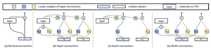
3.1.1 Hyper-Connections (HC)

The authors of the HC paper in 2025 stated that in the widely used residual connections (or skip connections as we commonly call it), there are “trade-offs between gradient vanishing and representation collapse”.

Here, the authors talk about ‘Pre-Norm’ and ‘Post-Norm’. In Pre-Norm, the input x is normalized before each residual block, ie. x + F(Norm(x)), while in Post-Norm, it is Norm(x + F(x)).

We know that residual connections were introduced in 2016 to mitigate the vanishing gradient problem. That is the Pre-Norm approach, which potentially suffers from representation collapse, where “hidden features in deeper layers become highly similar, diminishing the contribution of additional layers”. On the other hand, the Post-Norm approach is still prone to the vanishing gradient problem.

Hence, instead of adding an identity mapping with either pre- or post-Norm, the authors of HC propose learnable depth-connections and width-connections.

Screenshot of Figure 2 of Hyper Connections paper by Zhu et al. (2025) https://arxiv.org/pdf/2104.09864. Under (b), the hyper-connections enable lateral information exchange and vertical integration of features across depths.

Some people might feel a little uncomfortable seeing math like this.

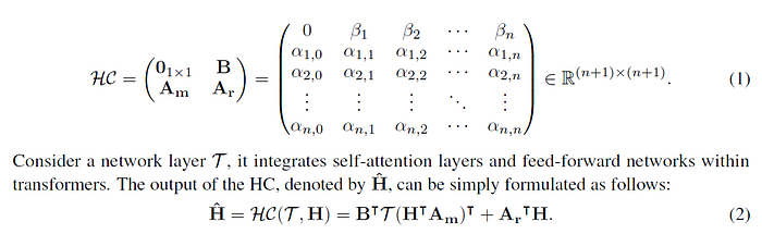Screenshot of equations (1) and (2) of Section 2.1 of Hyper Connections paper by Zhu et al. (2025).

However, once you expand the matrix out, using n=2 (it’s a small number, and also corresponds to the Figure 2), it’s not too bad. α and β are scalars, h₁ has shape (d, 1), as clearly stated in the first line of section 2.1 of https://arxiv.org/pdf/2104.09864.

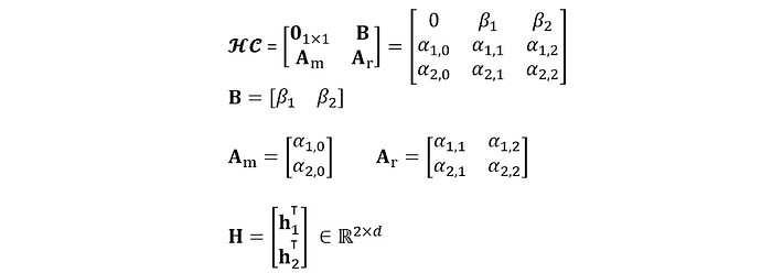Equation expanded and typed by author, based on equation (1), and the first paragraph of section 2.1 (for H), of Hyper Connections paper.

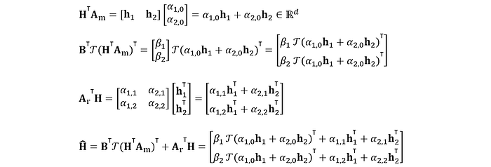
Therefore, the output of HC, as given by equation (2), works out to be

Equation expanded and typed by author, based on equation (2) of Hyper Connections paper.

This equation is just Figure 2(b) of the paper, written in math. Basically, what we have is this: take a weighted combination of h₁ and h₂, pass it through network layer calligraphic T, weight that output with β, and then add that to some other weighted combinations of h₁ and h₂.

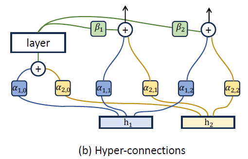Screenshot of Figure 2(b) of Hyper Connections paper by Zhu et al. (2025) https://arxiv.org/pdf/2104.09864.

The superscript to h is dropped, but h⁰ is just the initial input while hᵏ is the input to the (k+1) layer, where h₁⁰ and h₂⁰ are just replicas of h⁰.

This ‘layer’ itself could correspond to a block that includes attention and MoE. The left of the bottom figure shows where the original skip connections exist within multiple transformer blocks, while the right of the bottom figure shows HC in its place. Here, the However, note that the blocks in DeepSeek-v4 is NOT the simply the transformer block in DeepSeek-v3 with the residual connections replaced with the above.

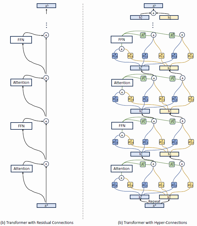Screenshot of Figure 8 of Hyper Connections paper https://arxiv.org/pdf/2104.09864.

3.1.2 Manifold-Constrained Hyper-Connections (mHC)

Now, we’re ready to jump into mHC proper.

In DeepSeek-v4 section 2.2, the authors wrote that using HC, “training will frequently exhibit numerical instability when stacking multiple layers”.

Let’s focus on the cited paper where mHC was first introduced (Xie et al. 2026). It is also a work by the DeepSeek organization. mHC was presented by Xie et al. as a means to mitigate the “risks of instability” as training scale increases.

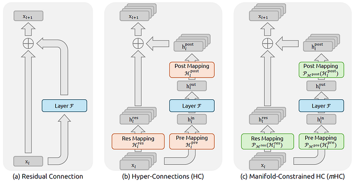Screenshot of Figure 1 of mHC paper by Xie et al. (2026). Unlike the unconstrained HC (b), mHC (c) focuses on optimizing the residual connection space by projecting the matrices onto a constrained manifold.

mHC expands the residual stream into multiple residual channels. Before each Transformer block, the channels are mixed into a d-dimensional input, and after, the output is written back into the expanded residual state. Hence, flexibility is increased, without increasing the hidden dimension.

What’s with the “Manifold-Constrained”? Well, it constrains the residual mixing matrix onto a specific manifold, as described by Equation (6) below, which almost looks mythical.

Screenshot of equation (6) of mHC paper by Xie et al. (2026). https://arxiv.org/pdf/2512.24880

Let’s break it down. The calligraphic Hₗʳᵉˢ with superscript ʳᵉˢ and subscript ₗ is the residual hyper-connection matrix at layer l, which the authors stated “represents a learnable mapping that mixes features within the residual stream” (section 1). Hₗʳᵉˢ is itself mathematically obtained from equation (5) of that paper.

We start with the simplest part, just the matrix alone. The component below means that the matrix of residuals has shape (n, n), where all values are real and non-negative.

Equation component typed by author

Since Xie et al. (2026) stated that they implemented mHC with n=4 (section 4.3 of the paper), I will plug in this value directly. The first constraint of the mHC equation (Hₗʳᵉˢ1ₙ = 1ₙ) dictates that each row of Hₗʳᵉˢ sums to 1, while the second constraint (1ₙᵀHₗʳᵉˢ = 1ₙᵀ) dictates that each column sums to 1.

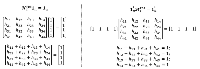Equation components typed by author, for 2nd and 3rd constraints of equation (6)

Collectively, all three constraints would mean that every stream distributes its weight fully, and every stream receives a total weight of 1. Values cannot be arbitrarily large, and every component Hₗʳᵉˢ would inevitably be bounded between 0 and 1. And that is it. You now understand what it means by restricting Hₗʳᵉˢ to be a “doubly stochastic matrix”.

3.1.3 mHC in DeepSeek-v4

Now, linking the above 3.3.1 (explaining HC) and 3.3.2 (explaining mHC) back to the DeepSeek-v4 paper.

Recall that in DeepSeek-v3, we have ordinary residual connections in each transformer block. (Figure 2 of https://arxiv.org/abs/2412.19437). In DeepSeek-v4, the authors recap (in section 2.2) that HC expands the residual stream from d to nₕ꜀×d, and that they used mHC to constrain the residual mapping matrix Bₗ to “the manifold of doubly stochastic matrices” M.

Screenshot of equation (2) of DeepSeek-v4 paper. https://huggingface.co/deepseek-ai/DeepSeek-V4-Pro/blob/main/DeepSeek_V4.pdf

There’s differences in the nomenclatures between those used by Zhu et al. (2025) and the DeepSeek-v4 authors, summarized in the table below.

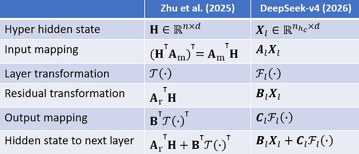Equations matched by author, comparing difference in nomenclatures

Meanwhile, Hₗʳᵉˢ in mHC of Xie et al. (2026) is represented as M in DeepSeek-v4.

Note that in DeepSeek-v4, Aₗ, Bₗ and Cₗ are actually not in boldface, but I find it a good habit to show matrices in bold. Also, Aₗ, Bₗ and Cₗ are dynamically generated, ie. they dependent on the input as well as other learnable parameters as given in equations (3) to (7) of the DeepSeek-v4 paper.

The model set-up details are specified in 4.2.1 of the DeepSeek-v4 paper. For V4-Pro, there are 61 Transformer layers, with hidden dimension d = 7168 and nₕ꜀ = 4.

3.2 Compressed Sparse Attention (CSA)

In the above section 3.1 of this article, we looked at the mHC, which is mainly about improving information flow and training stability for large context. In this section and the next, we focus on the aspects to “substantially reduce the computational cost of attention in long-text scenarios.”

3.2.1 DeepSeek Sparse Attention (DSA)

The predecessor to CSA is DSA, introduced in DeepSeek-v3.2 (2025). DSA contains a “Lightning Indexer” which scores how relevant prior tokens are to the current query (see equation 1 of section 2.1). Along with the ‘Top-k Selector’ (which the authors termed a “fine-grained token selection mechanism”), it selects the top-k key-value entries before applying attention.

Screenshot of Figure 2 of DeepSeek-v3.2 paper https://arxiv.org/pdf/2512.02556. Attention architecture where DSA is instantiated under MLA.

Based on my understanding (from section 2.1 of DeepSeek-v3.2), this “token selection mechanism” is really just a fanciful name for simply retrieving entries corresponding to top-k scores, which is straightforward conceptually as well as in terms of implementation.

For a quick comparison of this DSA differ from ordinary multi-head latent attention, I’ve include the screenshot of the MLA used in DeepSeek-v3. For more foundational knowledge of how DeepSeek-v3 works, refer to this guide by me.

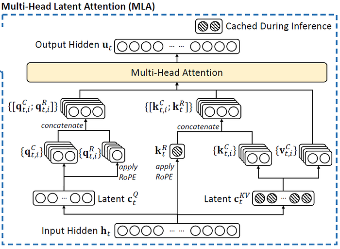Screenshot from the bottom-right portion of Figure 2 of Deepseek-v3 (2024) https://arxiv.org/pdf/2501.12948.

Notice that moving up from the input hidden state hₜ, the left side behaves in a similar manner where we have the latent cₜ𐞥 (the superscript should be Q, but unable to represent in-text), eventually leading to [qₜˏᵢꟲ; qₜˏᵢᴿ]. cₜ𐞥 is the shared compressed latent query representation for token t, while qₜˏᵢꟲ is the expanded content-query vector used by attention head i, while qₜˏᵢᴿ is its RoPE counterpart.

The right side is what differs. Both MLA and DSA still have the latent cₜᴷⱽ which is a compact cache that will allow subsequent reconstruction into kₜᶜ and vₜᶜ. But, in MLA of DeepSeek-v3, we have [qₜˏᵢꟲ; qₜᴿ] with [kₜˏᵢꟲ; kₜᴿ] and vₜˏᵢꟲ (across the multiple heads i) entering a multi-head attention for all past tokens. On the other hand, in DSA of DeepSeek-v3.2, the queries [qₜˏᵢꟲ; qₜᴿ] enter a multi-query attention just a subset of [cₜᴷⱽ; kₜᴿ] (corresponding to only the tokens selected by the ‘Top-k Selector’) and not all tokens. From cₜᴷⱽ, the k and v can be reconstructed, and in multi-query attention, the latent KV is shared across multiple queries for computational efficiency.

3.2.2 CSA in DeepSeek-v4

We can think of CSA as DSA applied to compressed KV blocks (rather than individual KV entries), with a local sliding-window branch added back for fine details.

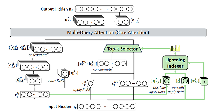
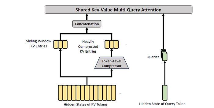
Screenshot of Figure 3 of DeepSeek-v4 paper, showing the core architecture of CSA.

To start off, consider H (a sequence of input hidden states, with sequence length n and hidden size d), represented by the bottom-left of the above figure. Within the Token-Level compressor, we have the following.

Cᵃ and Cᵇ are two token-level latent KV-entry streams produced by projecting the hidden sequence H through two different learned matrices Wᵃᴷⱽ and Wᵇᴷⱽ (equation 9), respectively, while Zᵃ and Zᵇ provide the logits (equation 11). Each m set of these gets compressed into one KV entry (equation 12). Recall that we had cₜᴷⱽ in MLA (DeepSeek-v3) and DSA (DeepSeek-v3.2). Here, we have two streams to allow information from overlapping windows to be combined into Cᶜᵒᵐᵖ, to reduce boundary artifacts and mitigate problems of possible ‘bad splits’.

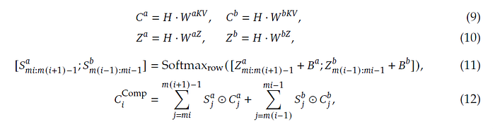Screenshot of equations (9) to (12) of DeepSeek-v4 paper.

⊙ in equation (12) denotes the Hadamard product (element-wise product of each matrix entry), while the softmax operation is performed along the row dimension comprising elements from both Zᵃ and Zᵇ. The added components Bᵃ and Bᵇ are learnable position biases.

CSA includes a component called Lightning Indexer (dotted box in Figure 3) for sparse selection (see equations 13 to 17 of section 2.3.1 of DeepSeek-v4).

As stated in 4.2.1 of the DeepSeek-v4 paper, for V4-Pro, the compression rate 𝑚 = 4, indexer query heads 𝑛ᴵₕ = 64, the indexer head dimension 𝑐ᴵ = 128, and the attention top-k is set to 1024. This means that for 1 million tokens, there would still be 250,000 Cᶜᵒᵐᵖ, and with sparse selection we keep to top 1024.

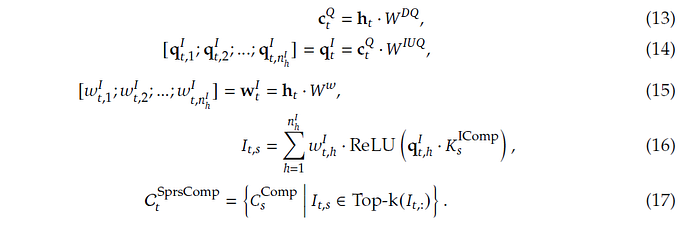Screenshot of equations (13) to (17) of DeepSeek-v4 paper.

Wᴰ𐞥 and Wᴵᵁ𐞥 (again, 𐞥 should be superscript Q which I am unable to present in-text) are learnable matrices, of shapes (d, d꜀) and (d꜀, cᴵnᴵₕ) respectively, which projects the input hidden state hₜ into qₜᴵ. (see equations 13 and 14). The use of Wᴰ𐞥 with Wᴵᵁ𐞥 is analogous to low-rank factorization, making the projection operation computationally cheaper. qₜᴵ is the indexer query used for sparse selection, containing concatenated information from across indexer heads. (An indexer head is different from an attention head, but the idea remains to have multiple ‘viewpoints’, in this case for scoring to subsequently determine selection).

Here comes the tricky part that is not explicitly written out mathematically. How is Kₛᴵᶜᵒᵐᵖ (on the RHS of equation 16) even obtained in the first place?

It is written that “CSA performs the same compression operation used for Cᶜᵒᵐᵖ to get compressed indexer keys Kᴵᶜᵒᵐᵖ” (equations 9 to 12, likely on different learned projection matrices).

Meanwhile, wₜᴵ corresponds to the weights for the indexer heads (equation 15), and the index score Iₜₛ is obtained (equation 16) from query token t and a preceding compressed block s. In equation 17, we get Cₜˢᵖʳˢᶜᵒᵐᵖ which is a subset of compressed KV entries (refer back to Figure 3 of DeepSeek-v4, on the arrows pointing into, and out of, the Top-k Selector) for those whose score Iₜₛ is within the top-k.

Finally, Cₜˢᵖʳˢᶜᵒᵐᵖ “serves as both attention key and value”, and enters Multi-Query Attention (MQA), with qₜ as the query (equation 19 of DeepSeek-v4 paper).

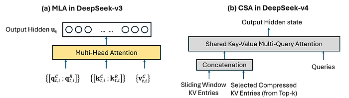Figure drawn by author, on the final inputs entering the multi-head/multi-query attention, taking reference to Figure 2 of Deepseek-v3, for (a), Figure 3 of DeepSeek-v4 paper, for (b).

Having a side-by-side comparison between MLA (of v3) and CSA (of v4), we see that the concatenation of {sliding window KV entries} and {selected compressed KV entries from top-k} in CSA serves the role of the attention memory that, in MLA, is represented by {[kₜˏᵢᶜ ; kₜˏᵢᴿ]} and {vₜˏᵢᶜ}. The sliding-window in DeepSeek-v4 is the most-recent 128 original uncompressed tokens.

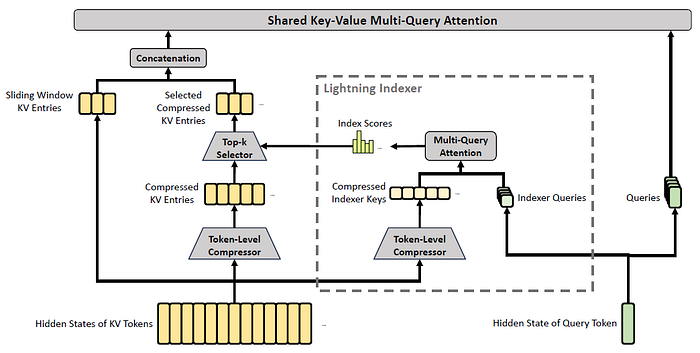
3.3 Heavily Compressed Attention (HCA)

The good (?) news is that we can jump straight-in without referring to another paper. This is unlike mHC, where we had to start with HC (3.1.1), nor like CSA, where we had to start with DSA (3.2.1).

The idea of HCA is to give the model a global view of the long context without too much computational costs, by performing attention over all the heavily compressed sequences. It “compresses the KV cache in a heavier manner, but does not employ sparse attention”. In a way, HCA is like a more extreme counterpart of CSA, where it selects only one of the two cost-saving aspects, and take it to the extreme.

Screenshot of Figure 4 of DeepSeek-v4 paper, showing the core architecture of HCA.

As stated in section 2.3.2, HCA employs a larger compression rate while not performing overlapped compression. The math (equations 20 to 23) is therefore very similar to equations (9) to (12).

In DeepSeek-v4, the compression rate m’ is 128 for HCA (instead of 4 in CSA). Therefore, suppose there are 1 million context tokens, HCA attends to 1000000/128 ~= 7,800 compressed KV entries Cᵢᶜᵒᵐᵖ (note that i refers to block index and not attention head), without any top-k selection. And unlike CSA which has two KV-entry streams with overlapping windows, there is only one stream here (boundary precision is less central here, since HCA is intended to provide a coarser global memory.).

Fine local details can also be handled by the sliding-window branch (containing uncompressed KV entries) which is concatenated to the heavily compressed (hence coarse) blocks.

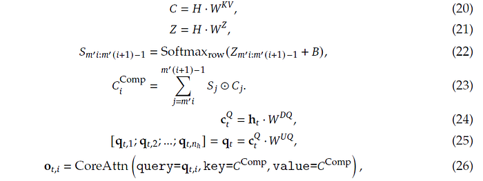Screenshot of equations (20) to (26) of DeepSeek-v4 paper, stitched together for compact presentation. Note that the key/value args within equation (26) has been written in a relaxed notation, because apart from Cᶜᵒᵐᵖ there should also be the non-compressed sliding-window entries, as mentioned in page 13 of the paper.

Like in CSA, attention queries are then obtained by low-rank projections (equation 24 and 25), and thereafter shared key-value multi-query attention is performed (equation 26), where multiple query heads attend to the same shared KV entries for efficiency.

As stated in 4.2.1 of the DeepSeek-v4 paper, CSA and HCA are used in an interleaved manner, and for both, the number of query heads 𝑛ₕ = 128, head dimension 𝑐 = 512, and the dimension of each intermediate attention output is 1024.

oₜˏᵢ computed from equation (26) is the core attention output of head i at token t. If we concatenate all head outputs, the dimensions will be 128 × 512 = 65536 which is large. Hence it is split into g=16 groups, with each projected into a 1024-dimensional intermediate output oₜˏᵢᴳ′. Finally, [oₜˏ₁ᴳ′ ; oₜˏ₂ᴳ′ ; … ; oₜˏ₁₆ᴳ′] are projected to the final attention output.

The DeepSeek-v4 authors also noted (in section 2.3.3) that before the core attention operation (MQA), RMSNorm is performed “on each head of the queries and the only head of the compressed KV entries”, and for each query and KV entry vector, they “apply RoPE to its last 64 dimensions”.

3.4 Muon optimizer

The muon optimizer has been introduced back in 2024, in an online post by Jordan, although it is not a formal academic paper or conference proceeding. (Then again, DeepSeek-v4 is also released as a technical report rather than academic paper or conference).

Now, you can simply run the Muon optimizer from Pytorch.

The name comes from MomentUm Orthogonalized by Newton-Schulz. Was not expecting that, and with this, I won’t be picturing Muon as an unstable subatomic particle in my mind now.

Muon optimizes neural network by “taking the updates generated by SGD-momentum, and then applying a Newton-Schulz (NS) iteration … before applying them to the parameters”. Implementation of NS is just a couple of lines of code.

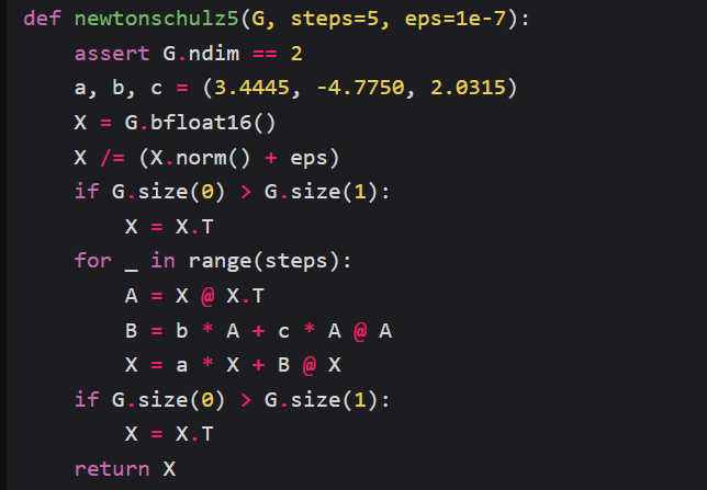Screenshot from Jordan (2024) https://kellerjordan.github.io/posts/muon/

Jordan (2024) clarified that Muon differs from Orthogonal-SGDM, in that it “moves the momentum to before the orthogonalization which performs better empirically”, and “uses a NS iteration instead of SVD” for efficiency. Earlier works were cited, along with alternatives for orthogonalizing matrix, a proof that NS iteration works (basically by transforming its singular values toward 1, thereby moving the matrix toward its orthogonal factor UVᵀ, without computing the SVD), and empirical observations. But we’ll not go down the rabbit hole, and instead move on to understand how it is applied.

For a deeper explanation of SVD, refer to Singular Value Decomposition — Explained with code. For concrete numbers on how gradient descent works, refer to my worked example on updating weights by gradient descent (which also has thousands of reads).

Here’s how Muon works at the high level. It looks very palatable when you put it side-by-side with something you already know, like SGD with momentum.

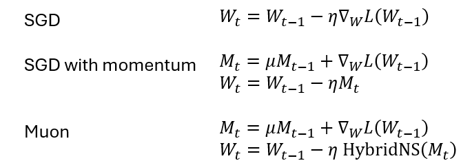Equations for SGD without and with momentum, and Muon (simplified at the high level, with details encapsulated within the NS operator). W refers to the trainable parameters ie. network weights, while M refers to the momentum.

In DeepSeek-v4, the authors stated that they implement hybrid NS with 10 iterations over two distinct stages (with specific combinations of coefficients a, b and c), for driving rapid convergence and then stabilizing the singular values. The pseudocode for implementation is as follows:

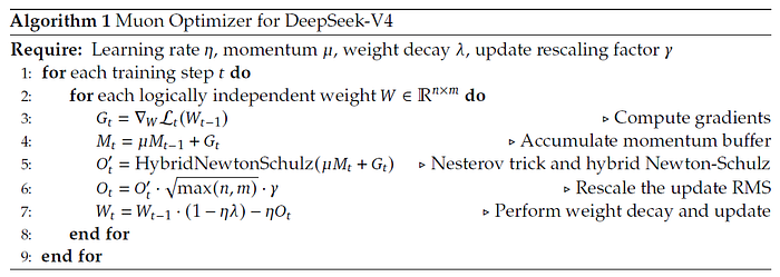Screenshot of Algorithm 1 of DeepSeek-v4 paper.

The ‘Nesterov trick’ in line 5 refers to computing gradients at the look-ahead rather than current parameters. The ‘Rescale update RMS’ in line 6 is as such because for a semi-orthogonal matrix in ℝⁿˣᵐ, its entries have RMS equal to 1/sqrt(max(n,m)). (A matrix is semi-orthogonal if its columns or rows are orthonormal. The RMS can be derived in a couple of lines.)

The DeepSeek-v4 authors wrote that AdamW (Adam with decoupled weight decay) optimizer was used for the embedding module, prediction head, mHC and weights of RMSNorm modules, while all others are updated with Muon.

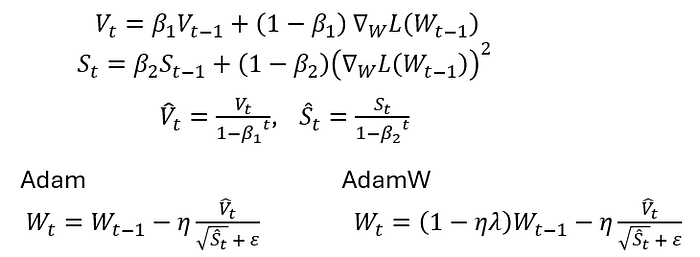Equations for Adam and AdamW, by author. Note that it is common for sources to refer to the first moment as m and second moment as v. However, I will use M and S instead, to be consistent with the above, M for ‘momentum’ (or first moment) and S for ‘second moment’ (helpful to remember squared too).

3.5 Infrastructures and Post-Training

There are also many other clever engineering aspects that makes DeepSeek-v4 possible, and we won’t be able to replicate anything similar at home. There’s another 29 pages of contents for sections 3, 4 and 5 of the DeepSeek-v4 paper, and this is where I draw the line.

Looking at the author list in Appendix A.1 of the paper, there are 270 authors listed, just under ‘Research & Engineering’.

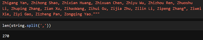Computation of number of authors under ‘Research & Engineering’.

No one in this world can convince me that this work would not have been possible if not for each and every one of the 270. But still, it’s clear that DeepSeek-v4 is the product of many brilliant minds working together. I don’t plan to touch things like “Expert Parallelism that fuses communication and computation” or “CUDA-based mega-kernel” or “translating TileLang’s integer expressions into Z3’s QF_NIA”. There’s simply too many other things to learn and to work on.

Conclusion

A year from now, these would probably be ‘old stuff’ in our fast-moving industry. However, I’m pretty confident that you’ll need to understand the concepts covered here as well as in the previous sections (on fundamentals) in order to keep up with the new developments.

This is the sort of guide I wish I had at the beginning, and now, I share them with you.

Disclaimer: All opinions and interpretations are that of the writer, and not of MITB. I declare that I have full rights to use the contents published here, and nothing is plagiarized. I declare that this article is written by me and not with any generative AI tool such as ChatGPT. I declare that no data privacy policy is breached, and that any data associated with the contents here are obtained legitimately to the best of my knowledge. I agree not to make any changes without first seeking the editors’ approval. Any violations may lead to this article being retracted from the publication.

Published in MITB For All 355 followers · Last published 1 day ago Tech contents related to AI, Analytics, Fintech, and Digital Transformation. Written by MITB Alumni; open-access for everyone.

Written by James Koh, PhD 1.2K followers · 54 following Data Science Instructor - teaching Masters students