Evaluating reasoning models
3 Evaluating reasoning models
This chapter covers
- Extracting final answers reliably from an LLM response
- Verifying answer correctness by comparing an LLM’s output to the reference solution using a symbolic math solver
- Running a full evaluation pipeline by loading a pre-trained model, generating outputs, and grading them against a dataset
Evaluation is what lets us distinguish between LLMs that merely sound convincing and those that can solve problems correctly. LLM evaluation techniques span a broad range of approaches, from measuring task accuracy to making sure that LLMs adhere to specific safety standards.
In this chapter, we focus on implementing a verification-based method that checks whether an LLM can solve math problems accurately by comparing its own answers against reference solutions using a calculator-like implementation.
This verifier is particularly useful because it not only evaluates performance on math tasks but also introduces the principle of verifiable rewards, which is the foundation of the reinforcement learning approach to reasoning models that we will implement later in chapter 6. (Interested readers can find additional evaluation methods in appendix F.)
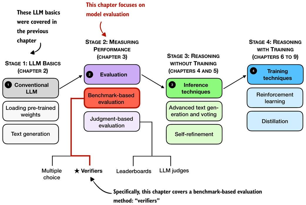 Figure 3.1 A mental model of the topics covered in this book. This chapter covers evaluation methods (stage 2), with a special focus on implementing verifiers.
3.1 Building a math verifier
There are four common ways of evaluating trained LLMs in practice: multiple choice, verifiers, leaderboards, and LLM judges, as shown in figure 3.1. These methods are widely used across research papers, technical reports, marketing materials, and model cards, and results often draw from more than one category.
As figure 3.1 illustrates, these evaluation approaches can be grouped into two broader types: benchmark-based evaluation and judgment-based evaluation. All four evaluation methods are useful in different contexts, but verifiers are especially relevant for reasoning models.
Math problems provide a natural example: depending on the problem complexity, math problems benefit from step-by-step reasoning to solve, the evaluation is straightforward because the final answer can be checked against a correct answer. In this setting, the verifier approach provides a simple and reliable way to measure whether a model’s reasoning steps lead to the correct outcome.
In this chapter, we focus on verifiers as a benchmark-based approach for measuring answer correctness in math problems, as illustrated in figure 3.2.
Note
For readers interested in going further, appendix F covers other evaluation methods such as multiple-choice benchmarks, preference-based leaderboards, and LLM-as-a-judge approaches.
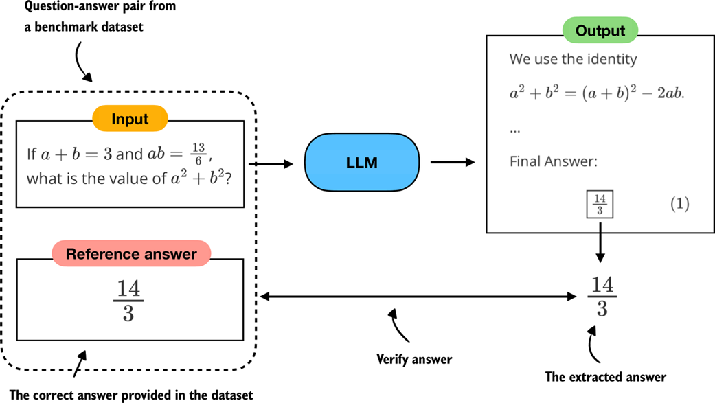 Figure 3.2 Evaluating an LLM with a verification-based method in free-form question answering. The model generates a free-form answer (which may include multiple steps) and a final boxed answer, which is extracted and compared against the correct answer from the dataset.
Verifiers compare the extracted answer with the reference solution, as shown in figure 3.2, often by relying on external tools such as code interpreters or calculator programs.
While our immediate focus is evaluation, verifiers will appear later in this book. They not only serve as a way to measure performance but also provide the feedback signal used in reinforcement learning methods for training reasoning models, which we will explore in chapter 6.
The downside is that verifier methods can only be applied to domains that can be easily (and ideally deterministically) verified, such as math and code. Also, this approach can introduce additional complexity and dependencies, and it may shift part of the evaluation burden from the model itself to the external tool.
However, because math problem solving can be generated in unlimited variations programmatically and benefits from step-by-step reasoning, this task has become a cornerstone of reasoning model evaluation and development.
In the remainder of this chapter, we will build a math verifier step by step, following the 8 steps shown in figure 3.3.
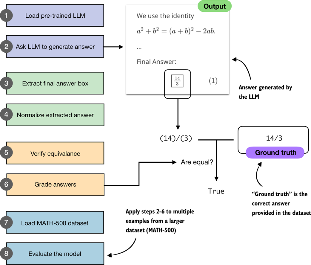 Figure 3.3 A step-by-step workflow for building and applying a math verifier. Starting with a pre-trained LLM, we generate answers, extract and normalize them, and then compare them against the ground-truth solutions. Verified answers are then graded, and the process is repeated across a dataset (MATH-500) to evaluate overall model performance.
The next section will start with steps 1 and 2 shown in figure 3.3, namely, loading the pre-trained LLM introduced in the previous chapter and setting it up to generate answers.
3.2 Loading a pre-trained model to generate text
In this section, we begin implementing the verifier by following steps 1 and 2 of the workflow in figure 3.3. Specifically, we will load the pre-trained LLM introduced in the previous chapter and configure it to generate answers. This provides the foundation for the later steps, where we will extract, normalize, and verify these answers.
Specifically, we use the same pre-trained base model that we used in chapter 2. However, for our convenience, and for reuse in future chapters, we wrap the model loading logic in a load_model_and_tokenizer function call as shown in listing 3.1:
Listing 3.1 Loading a pre-trained model
from pathlib import Path
import torch

from reasoning_from_scratch.ch02 import (
    get_device
)
from reasoning_from_scratch.qwen3 import (
    download_qwen3_small,
    Qwen3Tokenizer,
    Qwen3Model,
    QWEN_CONFIG_06_B
)


def load_model_and_tokenizer(
    which_model, device, use_compile, local_dir="qwen3"
):
    if which_model == "base":

        download_qwen3_small(
            kind="base", tokenizer_only=False, out_dir=local_dir
        )

        tokenizer_path = Path(local_dir) / "tokenizer-base.json"
        model_path = Path(local_dir) / "qwen3-0.6B-base.pth"
        tokenizer = Qwen3Tokenizer(tokenizer_file_path=tokenizer_path)

    elif which_model == "reasoning":

        download_qwen3_small(
            kind="reasoning", tokenizer_only=False, out_dir=local_dir
        )

        tokenizer_path = Path(local_dir) / "tokenizer-reasoning.json"
        model_path = Path(local_dir) / "qwen3-0.6B-reasoning.pth"
        tokenizer = Qwen3Tokenizer(
            tokenizer_file_path=tokenizer_path,
            apply_chat_template=True,
            add_generation_prompt=True,
            add_thinking=True,
        )

    else:
        raise ValueError(f"Invalid choice: which_model={which_model}")

    model = Qwen3Model(QWEN_CONFIG_06_B)
    model.load_state_dict(torch.load(model_path))

    model.to(device)

    if use_compile: # Optionally set to true to enable model compilation
        torch._dynamo.config.allow_unspec_int_on_nn_module = True
        model = torch.compile(model)

    return model, tokenizer


WHICH_MODEL = "base" # Uses the base model, similar to chapter 2, by default
device = get_device()
# device = torch.device("cpu") # Uncomment this line if you have compatibility issues with your device

model, tokenizer = load_model_and_tokenizer(
    which_model=WHICH_MODEL,
    device=device,
    use_compile=False
)
By default, listing 3.1 loads the base model, just as in chapter 2. An optional variant is the reasoning model, which the Qwen3 team trained on top of the base model using reasoning-specific methods. We will cover these training methods in chapter 6. Here, the reasoning model, which can be loaded by setting WHICH_MODEL = "reasoning" in listing 3.1, is included as an option so that we can later compare its evaluation results with those of the base model.
Now that we have loaded the model, we can use the text generation function from chapter 2 to generate text, as is shown in listing 3.2.
Listing 3.2 Generating model outputs
from reasoning_from_scratch.ch02 import (
    generate_text_basic_stream_cache
)

prompt = (
    r"If $a+b=3$ and $ab=\tfrac{13}{6}$, "
    r"what is the value of $a^2+b^2$?"
)

input_token_ids_tensor = torch.tensor(
    tokenizer.encode(prompt),
    device=device
).unsqueeze(0)

all_token_ids = []

for token in generate_text_basic_stream_cache(
    model=model,
    token_ids=input_token_ids_tensor,
    max_new_tokens=2048,
    eos_token_id=tokenizer.eos_token_id
):
    token_id = token.squeeze(0)
    decoded_id = tokenizer.decode(token_id.tolist())
    print(
        decoded_id,
        end="",
        flush=True
    )
    all_token_ids.append(token_id)

all_tokens = tokenizer.decode(all_token_ids)
In listing 3.2, we start by encoding a simple math problem into token IDs that the model can process. The model then generates tokens one by one in a streaming fashion, which we print immediately as they appear so we can read the output while it’s being generated. At the same time, we collect the generated tokens into a list so that we can later decode them into the complete final answer string. This pattern of both streaming and collecting tokens is handy because it lets us monitor the generation live while still storing the full answer text (all_tokens) that we can process later.
The response, generated by the code in listing 3.2, is as follows:
To find the value of \( a^2 + b^2 \) given that \( a + b = 3 \)
and \( ab = \frac{13}{6} \), we can use the following algebraic identity:

\[
a^2 + b^2 = (a + b)^2 - 2ab
\]

**Step 1:** Substitute the given values into the equation.

\[
a^2 + b^2 = (3)^2 - 2 \left( \frac{13}{6} \right)
\]

[...]

**Final Answer:**

\[
\boxed{\dfrac{14}{3}}
\]
As we can see, based on this answer, even though it is a base model, it provides a reasoning model-like explanation. This is likely because the Qwen3 team included chain-of-thought data during the pre-training stages, as stated in their technical report. However, even though the model has some reasoning-model-like behavior, adding additional reasoning methods can further improve these capabilities. (Note that the response may differ depending on whether you executed the code on a CPU, CUDA, or MPS device.)
Furthermore, if you are unfamiliar with the LaTeX syntax that is commonly used for mathematics, the response above can be very hard to decipher. If this is the case, you can use IPython’s Latex class to render it, as shown below:
from IPython.display import Latex, display
display(Latex(all_tokens))
Executing the code above in a code notebook will render the response as shown in figure 3.4.
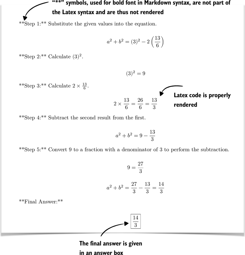 Figure 3.4 Rendered response with step-by-step calculations and the final boxed answer.
Note that the final answer given in figure 3.4,

is indeed the correct answer to this problem.
3.3 Implementing a wrapper for easier text generation
In the previous section, we loaded the pre-trained LLM and set up the text generation functionality (as illustrated in figure 3.5), which are the first two steps of the evaluation process covered in the remainder of this chapter.
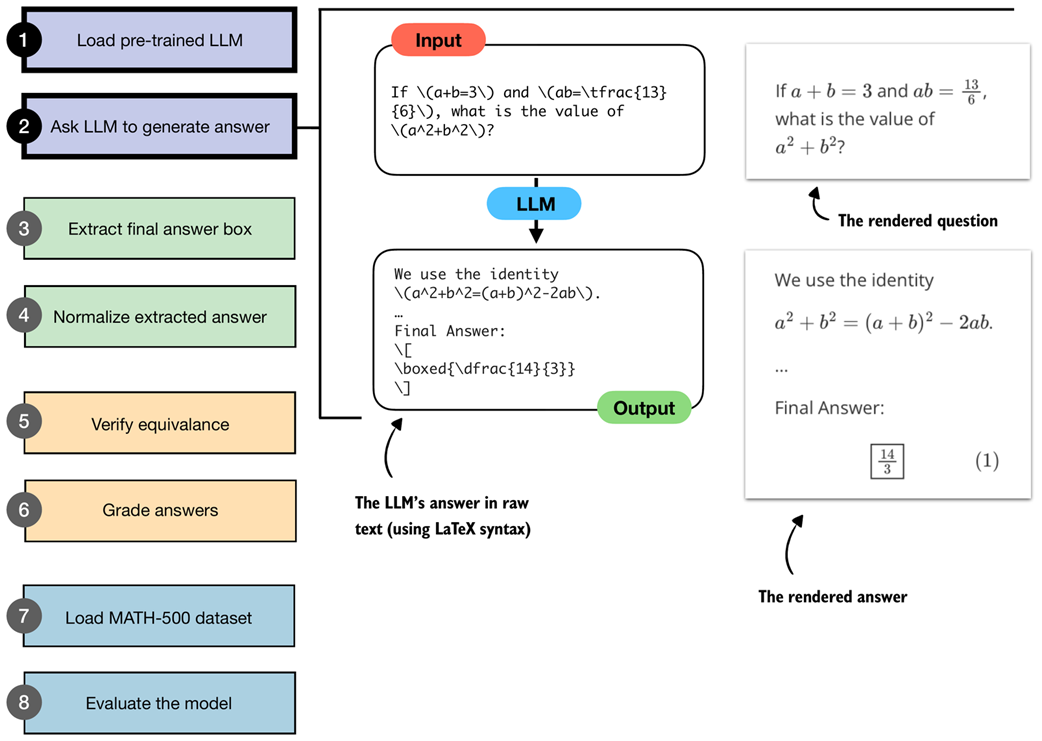 Figure 3.5 Illustration of steps 1 and 2 from the verifier workflow. A pre-trained LLM is loaded and prompted with a math problem, producing an output in raw LaTeX syntax. The answer is also shown in the rendered and more readable form.
For additional convenience in later sections, we create a wrapper (listing 3.3) for the text generation function so that we only have to pass in the model, tokenizer, and prompt, along with some additional settings instead of repeating the tokenization and input preparation steps each time:
Listing 3.3 A wrapper for streamed text generation
def generate_text_stream_concat(
    model, tokenizer, prompt, device, max_new_tokens,
    verbose=False,
):
    input_ids = torch.tensor(
        tokenizer.encode(prompt), device=device
        ).unsqueeze(0)

    generated_ids = []
    for token in generate_text_basic_stream_cache(
        model=model,
        token_ids=input_ids,
        max_new_tokens=max_new_tokens,
        eos_token_id=tokenizer.eos_token_id,
    ):
        next_token_id = token.squeeze(0)
        generated_ids.append(next_token_id.item())


        if verbose:
            print(
                tokenizer.decode(next_token_id.tolist()),
                end="",
                flush=True
            )

    return tokenizer.decode(generated_ids)
This wrapper function in listing 3.3 handles the full cycle of text generation: it tokenizes the input prompt, streams new tokens from the model, and then decodes the results into a final string. And, as mentioned before, the optional verbose flag allows us to see tokens as they are generated in real time. The function can be used as follows:
generated_text = generate_text_stream_concat(
    model, tokenizer, prompt, device,
    max_new_tokens=2048,
    verbose=True
)
This prints the exact same response as in section 3.2:
[...]

**Final Answer:**

\[
\boxed{\dfrac{14}{3}}
\]
3.4 Extracting the final answer box
Now that we have the model loaded and ready, we can get to the chapter-specific and interesting parts: evaluating the model.
Before we get started, it is worth recalling that this book takes a from-scratch approach, which naturally includes some detailed, sometimes tedious steps. This is intentional, since we want to build the evaluation pipeline ourselves to better understand how it works, rather than just calling predefined wrapper functions and building blocks.
In the previous section, we saw that the model returned the final answer in an answer box (written as r"\boxed{\dfrac{14}{3}}" in raw text), even though we hadn’t specifically asked for this format.
The reason the model answered in this specific format is likely because the model has seen examples from benchmark datasets (including MATH-500) that were similarly formatted during pretraining. This behavior is not necessarily proof of overfitting to the evaluation tasks we will run later. But it reflects that pre-trained models often encounter many problem formats online and learn to reproduce those stylistic conventions.
However, as a general rule, it is fair to assume that any information available on the internet when a model was trained has been part of the training data.
Although it was not necessary here, when we evaluate the model in the MATH-500 dataset later on, we will add a specific prompt that instructs the model to return answers in this boxed form, as it is a common convention that makes the evaluation more consistent across different models and makes data extraction easier.
We will now write code that performs this extraction of the boxed answer content as illustrated in figure 3.6.
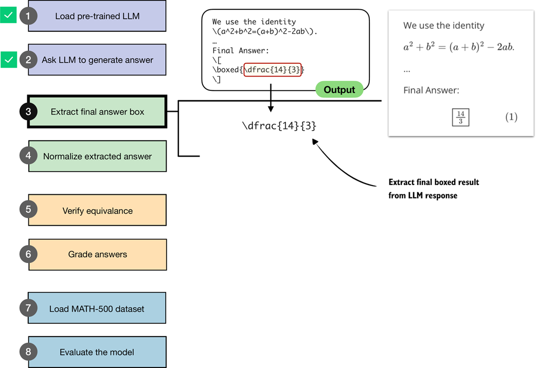 Figure 3.6 An illustration of how the boxed result from the LLM output is extracted.
Specifically, this section implements step 3 shown in figure 3.6. The next section will implement the normalization method for step 4.
Since your model may produce slightly different responses (depending on your hardware) than those shown above, we will work with a hard-coded answer for the time being (pretending that this answer was generated by the model). In later sections, we will revisit the model and have it generate answers for the tasks in the MATH-500 dataset.
model_answer = (
r"""... some explanation...
**Final Answer:**

\[
\boxed{\dfrac{14}{3}}
\]
""")
Note
We are using a raw string (
r"""..."""instead of a regular string"""..."""). Raw strings make it easier to handle the\character, which would otherwise be treated as escape sequences and require doubling backslashes.
Next, let’s define a function in listing 3.4 to extract the answer box from the model_answer.
Listing 3.4 Extracting answer boxes
def get_last_boxed(text):
    boxed_start_idx = text.rfind(r"\boxed")
    if boxed_start_idx == -1:
        return None

    current_idx = boxed_start_idx + len(r"\boxed")


    while current_idx < len(text) and text[current_idx].isspace():
        current_idx += 1


    if current_idx >= len(text) or text[current_idx] != "{":
        return None

    current_idx += 1
    brace_depth = 1
    content_start_idx = current_idx


    while current_idx < len(text) and brace_depth > 0:
        char = text[current_idx]
        if char == "{":
            brace_depth += 1
        elif char == "}":
            brace_depth -= 1
        current_idx += 1


    if brace_depth != 0:
        return None


    return text[content_start_idx:current_idx-1]
The get_last_boxed helper utility function in listing 3.4 extracts the content of the last \boxed{...} expression from a model’s output. More specifically, it scans for the final \boxed, skips over whitespace, checks for braces, and handles any nesting so that we capture the intended answer string.
While it may look a bit tedious, having this parser in place will pay off when we run evaluations on datasets like MATH-500, where extracting the correct final answer is the first step toward measuring a model’s reasoning ability. (MATH-500 is a curated collection of 500 problems that is widely used as a reasoning model benchmark dataset, which we will use later in this chapter.)
Now, let’s test it on the model answer:
extracted_answer = get_last_boxed(model_answer)
print(extracted_answer)
The output of this function call is "\dfrac{14}{3}", which is the boxed answer we wanted to extract.
Sidebar: Rendering math formulas
We can render math formulas via the
Latexclass we introduced earlier. Alternatively, for single math formulas that are not accompanied by answer text, we can also use the simpler Math class:from IPython.display import Math display(Math(r"\dfrac{14}{3}"))This renders the fraction as

While the previous get_last_boxed function correctly extracted the text, we will make the answer extraction a bit more robust to account for cases where a final answer box is either missing or incomplete via the extract_final_candidate function in listing 3.5:
Listing 3.5 Extracting the final answer candidate
import re

RE_NUMBER = re.compile(
    r"-?(?:\d+/\d+|\d+(?:\.\d+)?(?:[eE][+-]?\d+)?)"
)

def extract_final_candidate(text, fallback="number_then_full"):

    result = ""

    if text:
        boxed = get_last_boxed(text.strip())
        if boxed:
            result = boxed.strip().strip("$ ")


        elif fallback in ("number_then_full", "number_only"):
            m = RE_NUMBER.findall(text)
            if m:
                result = m[-1]
            elif fallback == "number_then_full":

                result = text
    return result
The extract_final_candidate function in listing 3.5 provides fallback settings in case no boxed answer can be found, which are as follows:
"number_then_full"(default): pick the last simple number, else the whole text;"number_only": pick the last simple number, else return an empty string"";"none": extract only boxed content, else return empty string"".
For the fallback setting, the code in listing 3.5 uses regular expressions (regex for short) via Python’s re library. Regexes are a way to search for patterns in text. In our case, the regex pattern is designed to recognize numbers, including fractions, decimals, and scientific notation. While the regex syntax looks intimidating, you don’t need to worry about the exact syntax here. What matters is that this gives us a reliable tool to extract the last numeric candidate from the model’s output when no boxed answer is available.
Let’s try it on our model answer:
print(extract_final_candidate(model_answer))
This correctly returns "\dfrac{14}{3}". Next, let’s try some additional examples. First, another boxed candidate:
print(extract_final_candidate(r"\boxed{ 14/3. }"))
This correctly returns "14/3.", stripping the extra whitespace but not the punctuation. However, the punctuation character will be handled correctly by the equality check we implement later.
Next, let’s try a candidate without a box, which should trigger the fallback setting, and see what happens:
print(extract_final_candidate("abc < > 14/3 abc"))
Thanks to the default fallback setting, it will find the last number in the answer and also correctly return "14/3".
In this section, we defined utility functions to extract the LLM’s answer from within its answer text content. This brings us one step closer to achieving the overall goal of verifying whether this answer is indeed correct. In the next section, we will normalize the response into a more general, canonical form before we implement the checking functionality.
Sidebar: Why not use an LLM for the answer extraction?
We could use an LLM itself to extract the boxed answer. However, this would introduce unnecessary complexity and potential errors. Extraction is a simple, mechanical task, assuming that the LLM outputs the answer in a specific format: we just need to locate the last boxed expression or, if that is missing, fall back to a number or the raw text.
Regular expressions may look complicated at first, but in the end, we have a small, reusable utility function that is cheap to execute and handles the extraction deterministically and reproducibly, without depending on the variability of another model’s output.
3.5 Normalizing the extracted answer
Previously, we extracted the boxed answer "\dfrac{14}{3}" from the model’s response. However, models may print the same value in many ways, such as "\frac{14}{3}", "14/3", "$14/3$", or "(14)/(3)". To implement and use a robust checking system that can check whether the answer is correct, we first need a consistent method of comparing results.
In this section, we implement a normalization (or canonicalization) pass (step 4 in figure 3.7) that strips formatting and standardizes the answer.
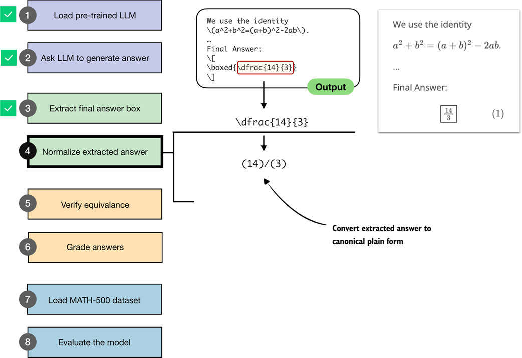 Figure 3.7 An illustration of how the boxed result from the LLM output is extracted and converted into a canonical plain form. This normalized answer is then later used for verification against the correct answer.
The normalization step shown in figure 3.7 is implemented via the normalize_text function in listing 3.6.
Listing 3.6 Normalizing extracted answers
LATEX_FIXES = [
    (r"\\left\s*", ""),
    (r"\\right\s*", ""),
    (r"\\,|\\!|\\;|\\:", ""),
    (r"\\cdot", "*"),
    (r"\u00B7|\u00D7", "*"),
    (r"\\\^\\circ", ""),
    (r"\\dfrac", r"\\frac"),
    (r"\\tfrac", r"\\frac"),
    (r"°", ""),
]

RE_SPECIAL = re.compile(r"<\|[^>]+?\|>")
SUPERSCRIPT_MAP = {
    "⁰": "0", "¹": "1", "²": "2", "³": "3", "⁴": "4",
    "⁵": "5", "⁶": "6", "⁷": "7", "⁸": "8", "⁹": "9",
    "⁺": "+", "⁻": "-", "⁽": "(", "⁾": ")",
}

def normalize_text(text):
    if not text:
        return ""
    text = RE_SPECIAL.sub("", text).strip()


    match = re.match(r"^[A-Za-z]\s*[.:]\s*(.+)$", text)
    if match:
        text = match.group(1)


    text = re.sub(r"\^\s*\{\s*\\circ\s*\}", "", text)
    text = re.sub(r"\^\s*\\circ", "", text)
    text = text.replace("°", "")

    match = re.match(r"^\\text\{(?P<x>.+?)\}$", text)
    if match:
        text = match.group("x")

    text = re.sub(r"\\\(|\\\)|\\\[|\\\]", "", text)


    for pat, rep in LATEX_FIXES:
        text = re.sub(pat, rep, text)


    def convert_superscripts(s, base=None):
        converted = "".join(
            SUPERSCRIPT_MAP[ch] if ch in SUPERSCRIPT_MAP else ch
            for ch in s
        )
        if base is None:
            return converted
        return f"{base}**{converted}"

    text = re.sub(
        r"([0-9A-Za-z\)\]\}])([⁰¹²³⁴⁵⁶⁷⁸⁹⁺⁻]+)",
        lambda m: convert_superscripts(m.group(2), base=m.group(1)),
        text,
    )
    text = convert_superscripts(text)


    text = text.replace("\\%", "%").replace("$", "").replace("%", "")
    text = re.sub(
        r"\\sqrt\s*\{([^}]*)\}",
        lambda match: f"sqrt({match.group(1)})",
        text,
    )
    text = re.sub(
        r"\\sqrt\s+([^\\\s{}]+)",
        lambda match: f"sqrt({match.group(1)})",
        text,
    )


    text = re.sub(
        r"\\frac\s*\{([^{}]+)\}\s*\{([^{}]+)\}",
        lambda match: f"({match.group(1)})/({match.group(2)})",
        text,
    )
    text = re.sub(
        r"\\frac\s+([^\s{}]+)\s+([^\s{}]+)",
        lambda match: f"({match.group(1)})/({match.group(2)})",
        text,
    )


    text = text.replace("^", "**")
    text = re.sub(
        r"(?<=\d)\s+(\d+/\d+)",
        lambda match: "+" + match.group(1),
        text,
    )


    text = re.sub(
        r"(?<=\d),(?=\d\d\d(\D|$))",
        "",
        text,
    )

    return text.replace("{", "").replace("}", "").strip().lower()
The normalize_text function in listing 3.6 takes an extracted answer string and rewrites it into a standardized format that we can reliably compare against reference solutions. It first strips away special tokens and unnecessary LaTeX clutter, such as \left, \right, or degree symbols. It then unwraps cases like \text{...}, removes inline math markers, and rewrites common structures into a calculator-style form. For example, it turns \sqrt{a} into sqrt(a) and \frac{a}{b} into (a)/(b). Finally, it normalizes exponents, mixed numbers, and thousands separators and cleans up braces and spacing. In short, the function transforms differently formatted LaTeX outputs into a clean, standardized string representation.
Let’s now try the normalize_text function on our model answer:
print(normalize_text(extract_final_candidate(model_answer)))
As a result, instead of printing the answer with LaTeX formatting (r"\dfrac{14}{3}"), it returns the answer in a standardized, LaTeX-free form:
"(14)/(3)"
Next, let’s try a differently formatted answer:
print(normalize_text(r"\text{\[\frac{14}{3}\]}"))
This also returns, "(14)/(3)", as intended.
We now have a robust method to extract answer texts from an LLM’s response. The next task, covered in the next section, is to implement a function to compare the LLM answer to a correct reference answer.
3.6 Verifying mathematical equivalence
So far, in this chapter, we implemented steps to ask an LLM to generate an answer, extract the relevant portion, and normalize it. The next step, as illustrated in figure 3.8, is to compare the extracted answer to a correct reference answer, which is, in technical contexts, referred to as ground truth.
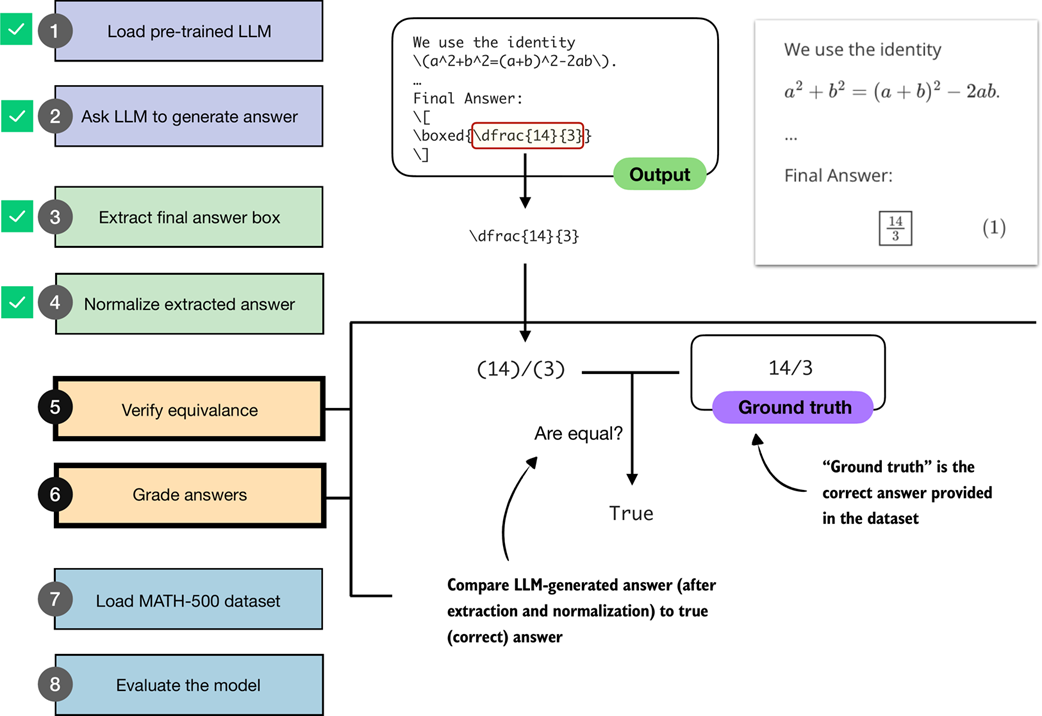 Figure 3.8 An illustration of how an LLM-generated answer is checked against the correct reference answer (ground truth). The final boxed answer is extracted and normalized, then compared to the correct answer provided in the dataset. If both match, the response is graded as correct.
Note that if we want to implement the equality check shown in figure 3.8, a direct comparison using Python’s == operator is not sufficient, since expressions like "14/3" and "(14)/(3)" would not match, and equivalent but unnormalized fractions such as "(28)/(6)" and "(14)/(3)" would also be treated as unequal.
As part of our equality check, we implement an additional intermediate step: parsing the extracted and normalized answer using a symbolic math engine.
For this, we use the SymPy open-source math library (https://sympy.org), which has been developed and tested for two decades and has become a staple of scientific computing in Python. The parsing function is implemented in listing 3.7.
Note
If you haven’t installed the dependencies in chapter 2, you can manually install SymPy via
uv pip install sympy(oruv add sympy).
Listing 3.7 SymPy parser for mathematical equality check
from sympy.parsing import sympy_parser as spp
from sympy.core.sympify import SympifyError
from sympy.polys.polyerrors import PolynomialError
from tokenize import TokenError

def sympy_parser(expr):
    try:
        return spp.parse_expr(
            expr,
            transformations=(
                *spp.standard_transformations,

                spp.implicit_multiplication_application,
            ),

            evaluate=True,
        )
    except (SympifyError, SyntaxError, TypeError, AttributeError,
            IndexError, TokenError, ValueError, PolynomialError):
        return None
The sympy_parser function in listing 3.7 takes an input expression, such as the normalized answer we extract from the LLM response, and converts it into a SymPy object that can be reliably compared for mathematical equivalence. To do so, it applies SymPy’s standard parsing rules, supports implicit multiplication like (2y instead of 2*y), and also simplifies basic arithmetic (so 2+3 becomes 5).
Note
The
sympy_parsertakes into account what looks like an excessive amount of error cases, but these are all errors that I encountered when evaluating the model on all 500 MATH-500 problems, as the model does not always generate perfectly formatted outputs.
Let’s see it in action and apply it to the normalized answer candidate:
print(sympy_parser(normalize_text(
    extract_final_candidate(model_answer)
)))
This returns the fraction 14/3. Next, let’s try an unnormalized fraction:
print(sympy_parser("28/6"))
Similarly, this returns 14/3.
Using the sympy_parser, we can now implement the equality check function in listing 3.8:
Listing 3.8 Equality check function using SymPy
from sympy import simplify

def equality_check(expr_gtruth, expr_pred):
    if expr_gtruth == expr_pred:
        return True


    gtruth, pred = sympy_parser(expr_gtruth), sympy_parser(expr_pred)

    if gtruth is not None and pred is not None:
        try:
            return simplify(gtruth - pred) == 0
        except (SympifyError, TypeError):
            pass

    return False
The equality_check function in listing 3.8 determines whether a model’s answer matches the ground-truth solution. It first looks for an exact string match, which is the simplest case. If the strings differ, it parses both expressions into SymPy objects (via the sympy_parser function we implemented in listing 3.7) and checks whether their difference simplifies to zero. This allows us to recognize answers that may look different on the surface (for example, 14/3 and 28/6) but are mathematically the same.
Let’s try the equality checker from listing 3.8 on an example:
print(equality_check(
    normalize_text("13/4."),
    normalize_text(r"(13)/(4)")
))
As intended, this ignores the formatting and returns True. Next, let’s try a more challenging example and see whether the symbolic math parser recognizes that 0.5 is the same as 1/2:
print(equality_check(
    normalize_text("0.5"),
    normalize_text(r"(1)/(2)")
))
This also returns True. Now, let’s try a negative example:
print(equality_check(
    normalize_text("14/3"),
    normalize_text("15/3")
))
This returns False since the expressions are different.
So far, so good. Based on the encouraging results above, we may conclude that we now have a robust equality checker that we can use to evaluate the LLM on a math benchmark dataset. However, to make sure that it’s ready for prime time, let’s try one more example:
print(equality_check(
    normalize_text("(14/3, 2/3)"),
    normalize_text("(14/3, 4/6)")
))
In this case, we are comparing two tuples. Since 2/3 and 4/6 are mathematically equivalent, we would expect the result to be True. Instead, the function returns False, because it currently only handles simple expressions, not tuples. We will address this limitation in the next section.
3.7 Grading answers
Now, we will build upon the mathematical equality checking function from the previous section to implement a robust grading function that can also handle tuple-like expressions, such as correctly comparing expressions like "(14/3, 2/3)" and "(14/3, 4/6)".
First, we implement a Python helper function that splits such tuple-like expressions into individual subparts via listing 3.9.
Listing 3.9 Helper function to split tuple-like expressions
def split_into_parts(text):
    result = [text]

    if text:
        if (
            len(text) >= 2
            and text[0] in "([" and text[-1] in ")]"
            and "," in text[1:-1]
        ):
            items = [p.strip() for p in text[1:-1].split(",")]
            if all(items):
                result = items
    else:
        result = []

    return result
The split_into_parts function in listing 3.9 helps us handle answers with multiple components. If the input looks like a tuple or list, such as (a, b) or [a, b], it splits the content on commas and returns the individual pieces. (If the string is empty, it simply returns an empty list.) In essence, this function breaks down multi-part answers into smaller parts that can be checked one by one.
Before we implement the grading function next, let’s take the split_into_parts for a test drive and try it on the tuple-like expression from earlier:
split_into_parts(normalize_text(r"(14/3, 2/3)"))
This returns ['14/3', '2/3'], as desired.
Now, we can implement the grade_answer function (listing 3.10), which splits tuple-like expressions (if present) into subparts, and then uses the equality_check function from the previous section to compare a generated answer to a reference (ground truth) answer.
Listing 3.10 Function to grade predicted answers against ground truth
def grade_answer(pred_text, gt_text):
    result = False
    if pred_text is not None and gt_text is not None:
        gt_parts = split_into_parts(
            normalize_text(gt_text)
        )
        pred_parts = split_into_parts(
            normalize_text(pred_text)
        )

        if (gt_parts and pred_parts
           and len(gt_parts) == len(pred_parts)):
            result = all(
                equality_check(gt, pred)
                for gt, pred in zip(gt_parts, pred_parts)
            )

    return result
The implementation of the grade_answer function in listing 3.10 first assumes the prediction is incorrect (False) and only continues if both prediction and ground truth are non-empty. It then normalizes each side and splits them into subparts (for example, breaking "(14/3, 2/3)" into ["14/3", "2/3"]). If the number of subparts matches, it compares them one by one using equality_check. The result is returned as correct (True) only if all pairs match mathematically.
We can think of the grade_answer function as an advanced version of the equality_check function from the previous section. The grade_answer function can split tuple-like expressions and normalize the answers before applying the equality_check function.
On simple expressions, it works similarly to the equality_check, returning True if two expressions are mathematically equivalent:
grade_answer("14/3", r"\frac{14}{3}")
In addition, as described above, it now also returns True in case of two mathematically equivalent tuple-like expressions:
grade_answer(r"(14/3, 2/3)", "(14/3, 4/6)")
To check the grade_answer function more comprehensively, the code in listing 3.11 contains more diverse test cases.
Listing 3.11 Test cases and demo function to test the grader
tests = [
        ("check_1", "3/4", r"\frac{3}{4}", True),
        ("check_2", "(3)/(4)", r"3/4", True),
        ("check_3", r"\frac{\sqrt{8}}{2}", "sqrt(2)", True),
        ("check_4", r"\( \frac{1}{2} + \frac{1}{6} \)", "2/3", True),
        ("check_5", "(1, 2)", r"(1,2)", True),
        ("check_6", "(2, 1)", "(1, 2)", False),
        ("check_7", "(1, 2, 3)", "(1, 2)", False),
        ("check_8", "0.5", "1/2", True),
        ("check_9", "0.3333333333", "1/3", False),
        ("check_10", "1,234/2", "617", True),
        ("check_11", r"\text{2/3}", "2/3", True),
        ("check_12", "50%", "1/2", False),
        ("check_13", r"2\cdot 3/4", "3/2", True),
        ("check_14", r"90^\circ", "90", True),
        ("check_15", r"\left(\frac{3}{4}\right)", "3/4", True),
        ("check_16", r"2²", "2**2", True),
    ]


def run_demos_table(tests):
    header = ("Test", "Expect", "Got", "Status")
    rows = []
    for name, pred, gtruth, expect in tests:
        got = grade_answer(pred, gtruth)
        status = "PASS" if got == expect else "FAIL"
        rows.append((name, str(expect), str(got), status))

    data = [header] + rows

    col_widths = [
        max(len(row[i]) for row in data)
        for i in range(len(header))
    ]

    for row in data:
        line = " | ".join(
            row[i].ljust(col_widths[i])
            for i in range(len(header))
        )
        print(line)

    passed = sum(r[3] == "PASS" for r in rows)
    print(f"\nPassed {passed}/{len(rows)}")
The code in listing 3.11 is a simple test suite that takes in a selection of tests to check whether the grade_answer function works as intended. The tests list contains tuples that cover a selection of fractions, LaTeX notation, tuple inputs, decimals, percentages, and other tricky formats.
The run_demos_table function then runs each test by calling grade_answer, collects the outcomes, and organizes the results into a formatted table.
Calling the run_demos_table(test) function in listing 3.11 prints the following:
Test     | Expect | Got   | Status
check_1  | True   | True  | PASS
check_2  | True   | True  | PASS
check_3  | True   | True  | PASS
check_4  | True   | True  | PASS
check_5  | True   | True  | PASS
check_6  | False  | False | PASS
check_7  | False  | False | PASS
check_8  | True   | True  | PASS
check_9  | False  | False | PASS
check_10 | True   | True  | PASS
check_11 | True   | True  | PASS
check_12 | False  | False | PASS
check_13 | True   | True  | PASS
check_14 | True   | True  | PASS
check_16 | True   | True  | PASS

Passed 16/16
As we can see based on the PASS results above, the grade_answer function is relatively robust and capable of handling a variety of differently formatted expressions.
Sidebar: Exercise 3.1: Adding more test cases
Try to think of additional test cases, ideally challenging ones, and add them to the
run_demos_table()function. Can you find cases where the check fails incorrectly?
With the grade_function implemented, we now have the building blocks in place to evaluate the LLM. In the next section, we will load a math dataset on which we will evaluate the LLM.
3.8 Loading the evaluation dataset
As we have seen in the chapter so far, implementing a robust verification pipeline can be a tedious task. Fortunately, we now have all the pieces in place, from answer extraction to grading, and are ready to evaluate the LLM on a benchmark dataset. For this, as illustrated in figure 3.9, we will use the MATH-500 dataset (https://huggingface.co/datasets/HuggingFaceH4/MATH-500), a widely used benchmark for reasoning models. It is a curated collection of 500 problems sampled from the original MATH dataset.
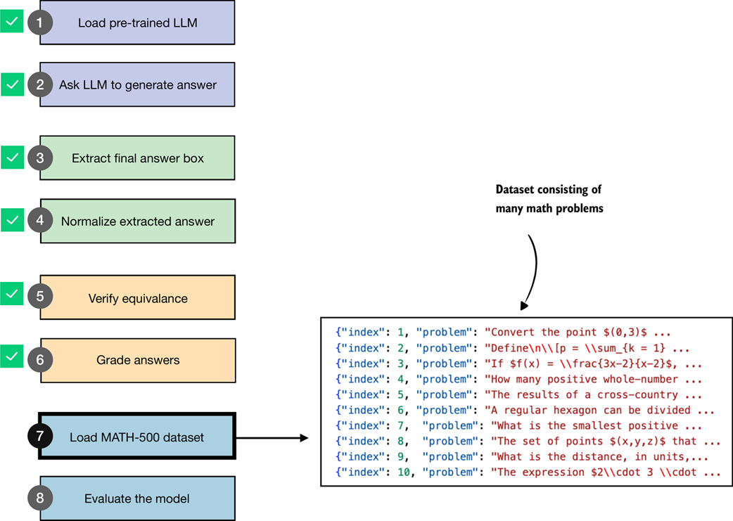 Figure 3.9 Loading the evaluation dataset. After completing steps 2–6 on individual problems (generate, extract, normalize, verify, and grade answers) in the previous sections, the two remaining steps are to load the full dataset (step 7) and apply the same procedure across all problems to evaluate the model (step 8).
We will load the MATH-500 dataset (step 7 in figure 3.9) using the following code:
Listing 3.12 Loading the MATH-500 dataset
import json
import requests

def load_math500_test(local_path="math500_test.json", save_copy=True):
    local_path = Path(local_path)
    url = (
        "https://raw.githubusercontent.com/rasbt/reasoning-from-scratch/"
        "main/ch03/01_main-chapter-code/math500_test.json"
    )

    if local_path.exists():
        with local_path.open("r", encoding="utf-8") as f:
            data = json.load(f)
    else:
        r = requests.get(url, timeout=30)
        r.raise_for_status()
        data = r.json()

        if save_copy:  # Saves a local copy
            with local_path.open("w", encoding="utf-8") as f:
                json.dump(data, f, indent=2)

    return data

math_data = load_math500_test()
print("Number of entries:", len(math_data))
This prints:
Number of entries: 500
Sidebar: Loading the dataset from Hugging Face Model Hub
The following information and code example is optional and provided for reference, and you don’t need to run the code below.
The MATH-500 dataset split was originally proposed in the PRM800K repository (https://github.com/openai/prm800k/tree/main?tab=readme-ov-file#math-splits) and is also available on the Hugging Face Hub (https://huggingface.co/datasets/HuggingFaceH4/MATH-500). However, in this book, we load a copy from the code repository to ensure reproducibility in case the external sources change.
If you prefer to download the dataset directly from Hugging Face, you can use the following code. Note that this requires the
datasetslibrary, which can be installed viapip install datasetsoruv add datasets:from datasets import load_dataset dset = load_dataset("HuggingFaceH4/MATH-500", split="test")
Before we jump to the next section to implement the model evaluation pipeline, let’s take a closer look at the structure of the dataset by printing its first entry (we use the built-in pprint library for nicer formatting):
from pprint import pprint
pprint(math_data[0])
This produces the following output:
{'answer': '\\left( 3, \\frac{\\pi}{2} \\right)',
 'level': 2,
 'problem': 'Convert the point $(0,3)$ in rectangular coordinates to polar '
            'coordinates.  Enter your answer in the form $(r,\\theta),$ where '
            '$r > 0$ and $0 \\le \\theta < 2 \\pi.$',
 'solution': 'We have that $r = \\sqrt{0^2 + 3^2} = 3.$  Also, if we draw the '
             'line connecting the origin and $(0,3),$ this line makes an angle '
             'of $\\frac{\\pi}{2}$ with the positive $x$-axis.\n'
             '\n'
             '[asy]\n'
             'unitsize(0.8 cm);\n'
             '\n'
             'draw((-0.5,0)--(3.5,0));\n'
             'draw((0,-0.5)--(0,3.5));\n'
             'draw(arc((0,0),3,0,90),red,Arrow(6));\n'
             '\n'
             'dot((0,3), red);\n'
             'label("$(0,3)$", (0,3), W);\n'
             'dot((3,0), red);\n'
             '[/asy]\n'
             '\n'
             'Therefore, the polar coordinates are $\\boxed{\\left( 3, '
             '\\frac{\\pi}{2} \\right)}.$',
 'subject': 'Precalculus',
 'unique_id': 'test/precalculus/807.json'}
As we can see, the dataset entry is formatted as a Python dictionary with keys and values. The relevant keys are
"problem": the math question or problem for the LLM to solve,"answer": the correct (ground truth) answer we want to compare the LLM answer against,"solution": a worked-out, step-by-step explanation of the problem (not used in this chapter, but useful for training or analysis).
(Note that the output contains the keys stored in alphabetical order: "answer", "problem", "solution", but the bulleted list uses the more logical ordering for readability.)
Now that we have a pre-trained LLM, evaluation functions, and a benchmark dataset to work with, we can implement the model evaluation.
3.9 Evaluating the model
In this section, we put the LLM text generation and evaluation tools from steps 2–6 in figure 3.10 into practice and apply them to the MATH-500 dataset (step 8 in figure 3.10), which we loaded in the previous section.
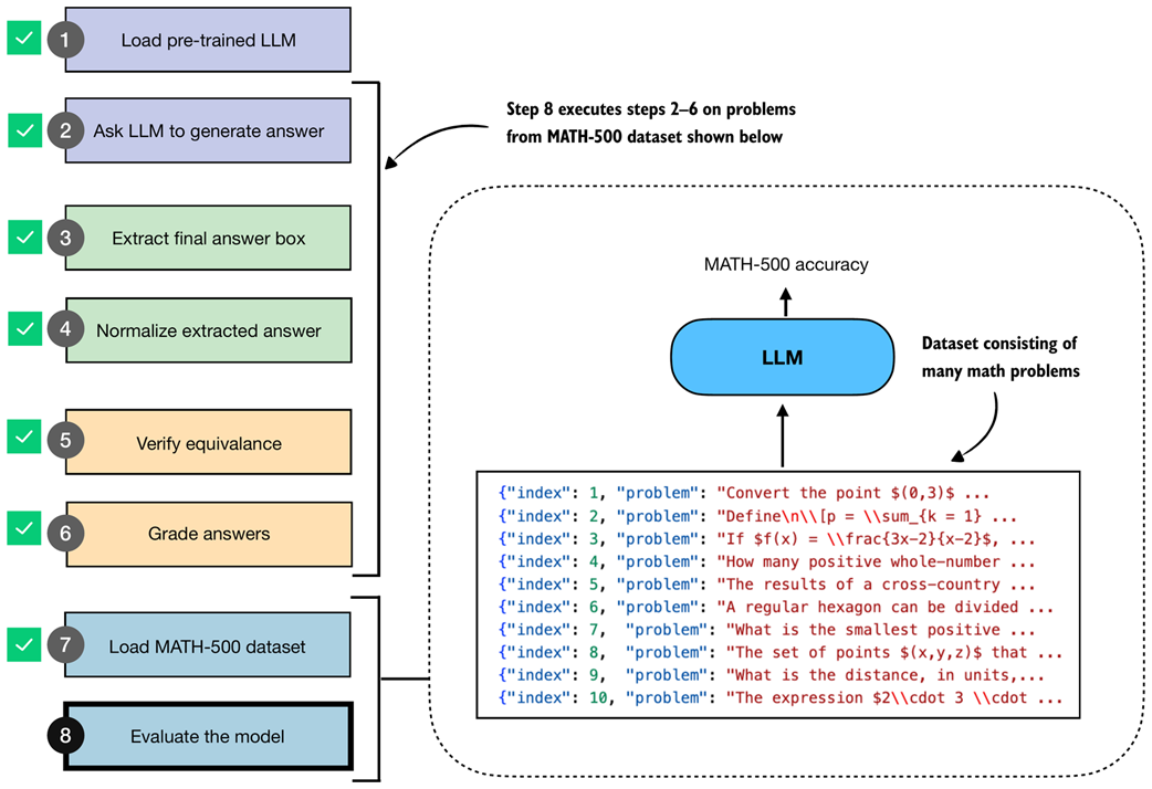 Figure 3.10 The complete evaluation pipeline on the MATH-500 dataset. After loading the dataset (step 7), steps 2–6 are applied systematically across all problems to obtain the final model evaluation (step 8).
As you may recall from section 3.4 (Extracting the final answer box), our answer checking pipeline expects that the model returns the answer in boxed form, which is a common convention when evaluating reasoning models on math problems. To increase the likelihood that the model adheres to this format, we can format the prompt as shown in listing 3.13:
Listing 3.13 Function to render a prompt template for math evaluation
def render_prompt(prompt):
    template = (
        "You are a helpful math assistant.\n"
        "Answer the question and write the final result on a new line as:\n"
        "\\boxed{ANSWER}\n\n"
        f"Question:\n{prompt}\n\nAnswer:"
    )
    return template
Let’s now apply the prompt template from listing 3.13 to the example prompt we introduced earlier in this chapter (section 3.2). For convenience, we redefine the example prompt here:
prompt = (
    r"If $a+b=3$ and $ab=\tfrac{13}{6}$, "
    r"what is the value of $a^2+b^2$?"
)
prompt_fmt = render_prompt(prompt)
print(prompt_fmt)
The formatted prompt is now as follows:
You are a helpful math assistant.
Answer the question and write the final result on a new line as:
\boxed{ANSWER}

Question:
If $a+b=3$ and $ab=\tfrac{13}{6}$, what is the value of $a^2+b^2$?

Answer:
Next, we pass the prompt to the text generation wrapper function we defined in listing 3.3 in section 3.3 to recap the text generation process before we construct the model evaluation function:
generated_text = generate_text_stream_concat(
    model, tokenizer, prompt_fmt, device,
    max_new_tokens=2048,
    verbose=True
)
Using this prompt example, the model responds with a relatively brief answer: "\boxed{10}". (Note that the generated response may differ depending on whether you executed the code on a GPU, CPU, or MPS device.)
While brevity can speed up generation by reducing the number of tokens, the response is incorrect. In contrast, in section 3.3, without a prompt template, the model produced a longer response, which led to the correct answer, 14/3.
However, whether a prompt template is well-suited for a given model and task ideally needs to be determined on a larger set of examples before we can draw any conclusions, for instance, the MATH-500 dataset we will evaluate the model on later in this section.
Sidebar: Prompt template choices
The prompt template in listing 3.13 is used here to demonstrate how a model evaluation pipeline can be implemented with answers that are automatically checked for correctness. The chosen template encourages short outputs, which lets you work through this chapter efficiently on a first read. Afterward, I recommend revisiting the chapter with alternative settings to optimize accuracy on the reasoning model variant.
As it turns out, using no prompt template boosts the base model performance by 50%, but it reduces the accuracy of the reasoning model by 40%.
Additionally, we may also experiment with alternative prompt templates. For instance, the common standard prompt for the MATH-500 benchmark is the following variant that swaps “Question:” with “Problem:” in listing 3.13. This seemingly minor change improves the base model’s accuracy by approximately 20%, likely because it better matches the memorized training data (assuming the MATH-500 test set was included in the training corpus). However, while the base model benefits from this change, the accuracy of the reasoning model variant drops by 30%.
Earlier, we mentioned that answer extraction is a simple, mechanical task that can be solved with deterministic code rather than employing another LLM for the answer extraction. Based on the accuracy change due to different prompting templates, it looks like our extraction method may not be reliable. However, this is not necessarily the case.
Also, it’s not necessarily the case that the LLM generates misformatted answers. It can just be incorrect, and switching to another LLM for extraction would not solve that. Smaller base models are often quite sensitive to prompt phrasing. In the next chapter, we will see how this becomes even more apparent once we introduce additional prompt variations.
Next, before we implement the final model evaluation function, let’s test our model evaluation pipeline end to end on a smaller example via the demo function in listing 3.14:
Listing 3.14 Demo function to run the evaluation pipeline
def mini_eval_demo(model, tokenizer, device):
    ex = {
        "problem": "Compute 1/2 + 1/6.",
        "answer": "2/3"
    }
    prompt = render_prompt(ex["problem"])
    gen_text = generate_text_stream_concat(
        model, tokenizer, prompt, device,
        max_new_tokens=64,
    )
    pred_answer = extract_final_candidate(gen_text)
    is_correct = grade_answer(
        pred_answer, ex["answer"]
    )

    print(f"Device: {device}")
    print(f"Prediction: {pred_answer}")
    print(f"Ground truth: {ex['answer']}")
    print(f"Correct: {is_correct}")
The mini_eval_demo function in listing 3.14 combines all the aspects we have covered so far in this chapter:
- Applying a prompt template
- Feeding the formatted prompt to the LLM to generate an answer
- Extracting and normalizing the answer
- Grading the answer
This mini_eval_demo function essentially connects the evaluation components together into a small function that we can use to test the code before coding the final evaluation pipeline for the MATH-500 dataset. The code starts from a raw example (ex), renders the problem into the prompt template (prompt), and streams a response from the model (generate_text_stream_concat). It then parses the model output to a final candidate answer (pred_answer) and grades it against the ground truth with grade_answer. Lastly, it prints the results for us to evaluate.
Calling the mini_eval_demo(model, tokenizer, device) function results in the following output:
Device: mps
Prediction: 1/3
Ground truth: 2/3
Correct: False
We can see that the generated answer ("1/3") was correctly extracted, but it doesn’t match the correct answer ("2/3"), and hence the check returns False. (Note that the results may differ depending on whether you execute the code on a CPU, CUDA, or MPS device.)
Now that we have tested our workflow on a simpler example, let’s implement it to run on the MATH-500 dataset.
Listing 3.15 End-to-end model evaluation pipeline for MATH-500 dataset
import time


def eta_progress_message(
    processed,
    total,
    start_time,
    show_eta=False,
    label="Progress",
):
    progress = f"{label}: {processed}/{total}"
    pad_width = len(f"{label}: {total}/{total} | ETA: 00h 00m 00s")
    if not show_eta or processed <= 0:
        return progress.ljust(pad_width)

    elapsed = time.time() - start_time
    if elapsed <= 0:
        return progress.ljust(pad_width)

    remaining = max(total - processed, 0)

    if processed:
        avg_time = elapsed / processed
        eta_seconds = avg_time * remaining
    else:
        eta_seconds = 0

    eta_seconds = max(int(round(eta_seconds)), 0)
    minutes, rem_seconds = divmod(eta_seconds, 60)
    hours, minutes = divmod(minutes, 60)
    if hours:
        eta = f"{hours}h {minutes:02d}m {rem_seconds:02d}s"
    elif minutes:
        eta = f"{minutes:02d}m {rem_seconds:02d}s"
    else:
        eta = f"{rem_seconds:02d}s"

    message = f"{progress} | ETA: {eta}"
    return message.ljust(pad_width)


def evaluate_math500_stream(
    model,
    tokenizer,
    device,
    math_data,
    out_path=None,
    max_new_tokens=512,
    verbose=False,
):

    if out_path is None:
        dev_name = str(device).replace(":", "-")
        out_path = Path(f"math500-{dev_name}.jsonl")

    num_examples = len(math_data)
    num_correct = 0
    start_time = time.time()

    with open(out_path, "w", encoding="utf-8") as f:
        for i, row in enumerate(math_data, start=1):
            prompt = render_prompt(row["problem"])
            gen_text = generate_text_stream_concat(
                model, tokenizer, prompt, device,
                max_new_tokens=max_new_tokens,
                verbose=verbose,
            )

            extracted = extract_final_candidate(
                gen_text
            )
            is_correct = grade_answer(
                extracted, row["answer"]
            )
            num_correct += int(is_correct)

            record = {
                "index": i,
                "problem": row["problem"],
                "gtruth_answer": row["answer"],
                "generated_text": gen_text,
                "extracted": extracted,
                "correct": bool(is_correct),
            }
            f.write(json.dumps(record, ensure_ascii=False) + "\n")

            progress_msg = eta_progress_message(
                processed=i,
                total=num_examples,
                start_time=start_time,
                show_eta=True,
                label="MATH-500",
            )
            print(progress_msg, end="\r", flush=True)

            if verbose:
                print(
                    f"\n\n{'='*50}\n{progress_msg}\n"
                    f"{'='*50}\nExtracted: {extracted}\n"
                    f"Expected:  {row['answer']}\n"
                    f"Correct so far: {num_correct}\n{'-'*50}"
                )

    seconds_elapsed = time.time() - start_time
    acc = num_correct / num_examples if num_examples else 0.0
    print(f"\nAccuracy: {acc*100:.1f}% ({num_correct}/{num_examples})")
    print(f"Total time: {seconds_elapsed/60:.1f} min")
    print(f"Logs written to: {out_path}")
    return num_correct, num_examples, acc
The evaluate_math500_stream function in listing 3.15 uses the same main steps as the smaller demo function from listing 3.14: for each problem, it renders the prompt, streams a model response, extracts the answer candidate, and grades it against the reference answer.
In addition to iterating over a dataset with multiple entries, it adds some additional bells and whistles. For instance, it saves the generated responses to a JSONL file in a Python dictionary-like format for record keeping and closer inspection.
Let’s now run this function on a subset, the first 10 examples of MATH-500, which takes about 0.7 minutes on a Mac Mini with an M4 chip. (Evaluating the reasoning model variant takes about 7 min as it generates longer responses.)
print("Model:", WHICH_MODEL)
num_correct, num_examples, acc = evaluate_math500_stream(
    model, tokenizer, device,
    math_data=math_data[:10],
    max_new_tokens=2048,
    verbose=False
)
In the code example above, we set max_new_tokens to a generous 2048, since the reasoning model variant, by design, tends to generate much longer responses, and we don’t want to cut it off prematurely. This, however, leads to much longer evaluation times, where it may appear that the generation is stuck. Optionally, you could set verbose=True to see the response being generated live, token by token.
The result of running the evaluate_math500_stream function is as follows:
Model: base
Device: mps
MATH-500: 10/10 | ETA: 00s
Accuracy: 30.0% (3/10)
Total time: 0.4 min
(Note that the results may differ depending on whether you execute the code on a GPU, CPU, or MPS device.)
As we can see, the model achieves a relatively low accuracy of 30%. We can open the math500_base-mps.jsonl file in a text editor to analyze the results, together with the generated response. For instance, we find that the answers, in all cases, have been successfully extracted, but they are plain wrong, which indicates that the model does not have very strong math problem-solving capabilities (yet). This is expected since it’s merely a base model.
Sidebar: Loading the .jsonl file programmatically
The
.jsonlfile suffix is a convention used for JSON files with one data entry per row. You can view it in your favorite text editor. Optionally, we can load the .jsonl file created during the evaluation in Python using the following code:dev_name = str(device).replace(":", "-") local_path = f"math500_{WHICH_MODEL}-{dev_name}.jsonl" results = [] with open(local_path, "r") as f: for line in f: if line.strip(): results.append(json.loads(line))
The reasoning model variant, which you can enable by setting WHICH_MODEL = "reasoning" in listing 3.1 in section 3.2, performs much better and achieves a 90% accuracy on the same 10-sample subset and 50.8% on the complete 500-sample dataset, as shown in table 3.1.
Table 3.1 MATH-500 task accuracy on different devices
| Mode | Device | Accuracy | MATH-500 size |
|---|---|---|---|
| Base | CPU | 30% | 10 |
| Base | CUDA | 30% | 10 |
| Base | MPS | 30% | 10 |
| Reasoning | CPU | 90% | 10 |
| Reasoning | CUDA | 90% | 10 |
| Reasoning | MPS | 80% | 10 |
| Base | CUDA | 15.3% | 500 |
| Reasoning | CUDA | 50.8% | 500 |
As shown in table 3.1, the reasoning variant, with its longer responses, has a drastically improved accuracy, but also increases the compute intensity and answer generation time substantially (from 0.4 min for the base model to 7 min for the reasoning model on a Mac Mini with M4 chip on the 10-sample subset, and from 13.3 min to 185.4 min on an H100 on the 500-sample dataset), which highlights one of the trade-offs of using reasoning models. Please note that these numbers were obtained in PyTorch 2.8 and can differ in different versions of PyTorch.
Tip
The code repository contains a bonus script (https://github.com/rasbt/reasoning-from-scratch/blob/main/ch03/02_math500-verifier-scripts/evaluate_math500_batched.py) that runs the code in this chapter in batched mode. This means it processes multiple examples per forward pass to accelerate the evaluation while requiring more RAM. With a batch size of 128, this reduces the runtime of the base model, when evaluating all 500 samples, from 13.3 min to 3.3 min on an H100 GPU. Similarly, it reduces the runtime of the reasoning model from 185.4 min to 14.6 min. Note that the H100 is used as an example, and the script is compatible with other GPUs as well.
Sidebar: Exercise 3.2: Calculating the average response length
Try to modify the code in this chapter to also report the average response length in the
evaluate_math500_streamfunction in listing 3.15. Instead of modifying the function directly, you could also compute the response length from the generated JSON report itself.
Sidebar: Exercise 3.3: Extending or changing the evaluation dataset
We choose a subset of only 10 examples for computational efficiency. However, readers are encouraged to consider running the code on larger or different portions of the dataset to observe whether the 10-sample subset is representative. Ideally, you could also experiment with your own data. (For reference, evaluating the base model on the complete MATH-500 dataset takes about 13.3 min for the base model and 185.4 min for the reasoning model on an H100.)
Sidebar: Exercise 3.4: Experimenting with different prompt templates
Models can be sensitive to different prompt templates. Experiment with different prompt templates in listing 3.13 to see how it affects the results. Also, while the Qwen3 team recommends using the base model without an additional chat template, you can additionally enable the
apply_chat_template=Truesetting in the tokenizer (listing 3.1) and observe whether it improves the base model performance.
Note that this concludes our chapter on implementing a verification-based approach for math tasks (figure 3.11). We chose math because it is both natural to implement and widely used in reasoning-specific training, particularly reinforcement learning with verifiable rewards, which we will cover in chapter 6. The same concept can be extended to other domains, such as code, although we did not explore that here since executing code would require additional setup of a secure virtual environment.
Before we move on, it is worth noting that evaluation also comes in many other flavors. In this chapter we focused on verification-based accuracy for math problems, as it is a popular method, and because we will reuse the same verifier as part of the reinforcement learning pipeline in chapters 6 and 7.
For a broader overview, appendix F walks through other common evaluation strategies, such as multiple-choice benchmarks, verifiers, leaderboards, and LLM-as-judge setups. This appendix provides an overview with hands-on examples if you want a quick tour of how these methods work in practice.
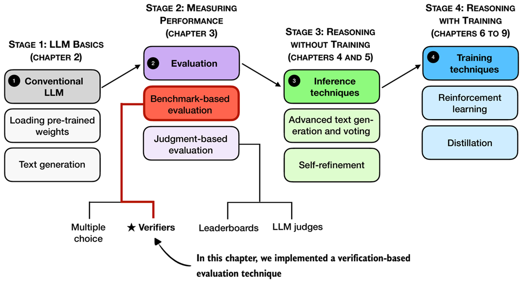 Figure 3.11 Mental model of the topics covered in this book. This chapter implemented a verifier-based evaluation pipeline. In the next chapter, we will improve the reasoning capabilities of the LLM via more advanced inference techniques.
Now, with an evaluation framework in place, the next chapter, as shown in figure 3.11, focuses on improving the reasoning capabilities through more advanced inference (text generation) techniques.
3.10 Summary
- There are four main evaluation methods for LLMs: multiple choice, verifiers, leaderboards, and LLM judges
- Verification-based evaluation methods allow free-form answers and use external tools to check correctness
- This chapter focuses on verification-based evaluation by building a math verifier that extracts, normalizes, and checks answers with SymPy
- The verification pipeline involves several core steps from loading the LLM to running the evaluation on a dataset
- As part of the verification pipeline, answer extraction uses string parsing to locate boxed content (with fallback mechanisms for missing boxes)
- Another step implements normalization, which standardizes diverse answer formats by stripping LaTeX and converting mathematical notation
- Finally, the pipeline uses mathematical equivalence checking (via SymPy) to compare expressions symbolically
- The MATH-500 dataset provides 500 curated math problems for evaluation
- Prompt templates significantly impact model performance
- The reasoning model achieves higher accuracy than the base model, but requires much longer runtime