Distilling reasoning models for efficient reasoning
8 Distilling reasoning models for efficient reasoning
This chapter covers
- Hard and soft distillation for reasoning models
- Creating and preparing a teacher-generated reasoning dataset
- Training and evaluating a distilled student model using cross-entropy loss
Reasoning performance can be improved not only through inference-time scaling and reinforcement learning, but also through distillation. In distillation, a smaller student model is trained on reasoning traces and answers generated by a larger teacher model. As shown in the overview in figure 8.1, this chapter focuses on this training-time technique.
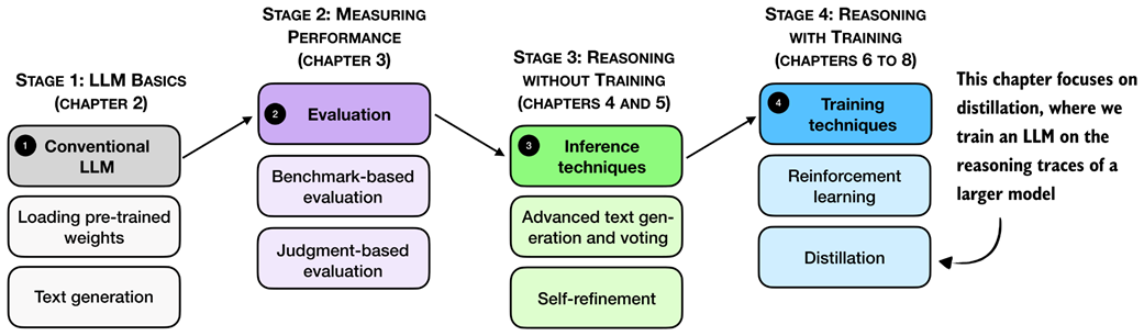 Figure 8.1 A mental model of the topics covered in this book. This chapter focuses on distillation, where a smaller student model is trained on reasoning traces generated by a larger teacher model.
First, we’ll take a look at a general introduction to model distillation before discussing the individual steps shown in figure 8.1 in more detail.
8.1 Introduction to model distillation for reasoning tasks
Model distillation means training a smaller LLM, the student, on outputs produced by a larger LLM, the teacher. For reasoning models, these outputs usually include not only the final answer but also the intermediate reasoning trace that leads to it.
Distillation is especially relevant because the strongest reasoning models are often too large and expensive to work with directly. For example, DeepSeek-R1 has 671-billion-parameters. Systems at that scale are expensive to develop, expensive to deploy, and far outside what most practitioners can run on local hardware.
This chapter is meant to help you make reasoning distillation happen at a smaller scale. You may recall DeepSeek-R1 created smaller model variants by distilling the 671-billion-parameter teacher model. We follow the same basic workflow, but at a scale that is practical for this book.
Throughout this book, we deliberately worked with small models rather than training a very large LLM from scratch. But the workflow in this chapter is still the same. We use a stronger teacher to generate reasoning traces, and then train a smaller student to reproduce them. In our setup, this distillation stage also takes only a fraction of the time. Here, the distillation training run takes about 3 hours on a GPU System using about 15 GB of VRAM, whereas even a few RLVR rounds in chapter 6 took around 12 hours and about 70 GB of VRAM on the same hardware.
Distillation can also be more effective than training a small model with reinforcement learning with verifiable rewards (RLVR) from scratch. For example, the DeepSeek-R1 paper reported that its smaller distilled variants outperformed comparable models trained with reinforcement learning alone. In that setup, the largest DeepSeek-R1 model, with 671 billion parameters, acted as the teacher and generated the supervision used to train smaller student models.
There are two main types of distillation: hard distillation and soft distillation. In hard distillation, the student is trained on text generated by the teacher, so the teacher’s tokens are treated as the targets. In soft distillation, the student is trained to match the teacher’s probability distribution over the vocabulary by minimizing the KL divergence, a measure of how different two probability distributions are. These two approaches are illustrated in figure 8.2.
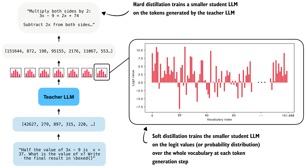 Figure 8.2 Hard distillation trains the student on teacher-generated tokens, soft distillation trains the student on the teacher’s full output distribution.
As illustrated in figure 8.2, one option is pure hard distillation. Here, we use only the teacher-generated text as the training target.
For those familiar with the typical LLM training pipeline, which is covered in more detail in my other book, Build a Large Language Model (From Scratch), hard distillation is just supervised fine-tuning on synthetic data.
This is also the setup used for the smaller DeepSeek-R1 distilled models. A large teacher model generates reasoning traces and answers, and the student model is fine-tuned to reproduce them.
According to the DeepSeek-R1 paper, for small models, this distillation approach can result in higher accuracy than training with reinforcement learning.
The main practical advantage of hard distillation is that we only need access to the teacher’s generated text, not its logits.
The second option is pure soft distillation. Instead of matching only the teacher’s chosen tokens, the student is trained to match the teacher’s full output distribution of each token over the whole vocabulary. This gives the student richer information about which alternative tokens the teacher considered plausible, but it requires access to teacher logits or log-probabilities at training time.
A third option combines hard and soft distillation. This is the classic knowledge-distillation setup popularized earlier in computer vision, for example in the paper Distilling the Knowledge in a Neural Network. In this case, we train on the teacher’s actual output tokens while also encouraging the student to match the teacher’s full distribution.
In practice, hard distillation is much more common for LLMs. One reason is that full teacher logits are usually inaccessible. Proprietary systems such as ChatGPT or Claude may expose generated text, but they generally do not expose the full vocabulary distribution needed for classical soft distillation.
Caution Reusing generated text for distillation may be restricted by provider-specific usage policies, including the OpenAI and Anthropic Terms of Service, so these should be reviewed carefully in practice before using such outputs for training.
Even when logits are available, soft distillation is more cumbersome. The student and teacher usually require the same tokenizer so that their vocabulary distributions line up, which makes this approach easier within the same model family. It is also much more expensive to store and use full token distributions for long reasoning traces. By comparison, storing plain text outputs is cheap and simple.
Here, we focus on hard distillation in the style of DeepSeek-R1 because it is the more practical setup for most readers. The chapter steps are summarized in figure 8.3.
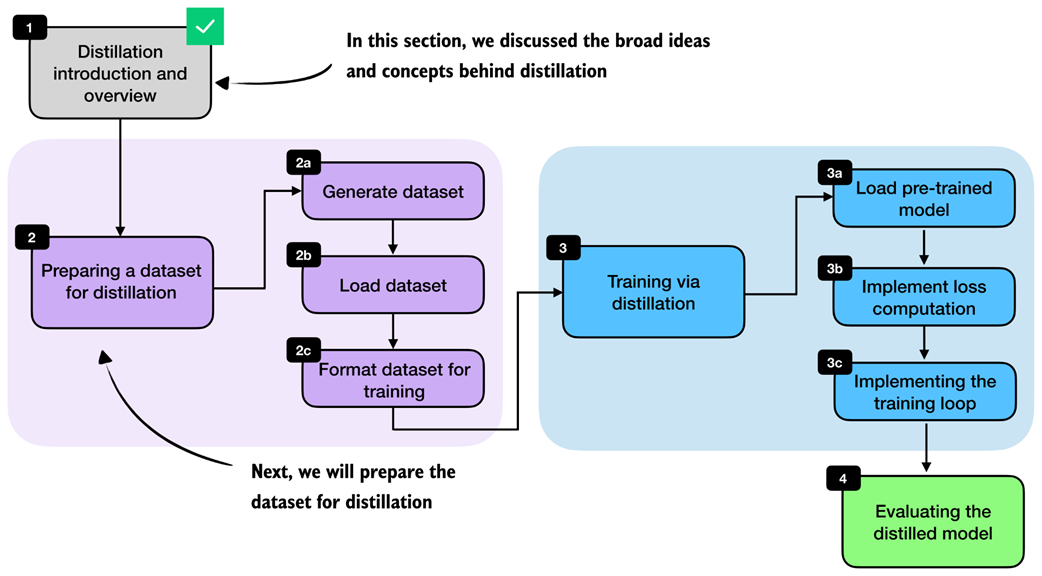 Figure 8.3 Chapter overview. After introducing the main distillation concepts, we generate and load a distillation dataset, format it for training, train the student model, and finally evaluate it.
With this overview in place, we can now move from the high-level ideas behind distillation to the practical steps required to implement it. In the next section, we begin by preparing a dataset for distillation, which serves as the foundation for training the student model.
8.2 Generating a dataset for reasoning distillation
The first practical step is to create a dataset for training the student model. For us, the student is again the Qwen3 0.6B base model that we used throughout the earlier chapters.
To build the dataset, we use the 12,000 math problems from the MATH split that do not overlap with the MATH-500 evaluation set. These are the same 12,000 problems that we used in chapters 6 and 7 for RLVR. Instead of sampling multiple student responses and computing rewards, however, we now feed these problems to an existing reasoning model, DeepSeek-R1, and collect its responses as training targets. This setup is illustrated in figure 8.4.
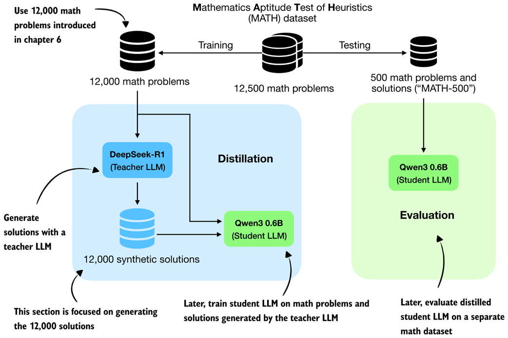 Figure 8.4 Distillation setup used in this chapter. We use the 12,000 non-overlapping MATH training problems to obtain synthetic solutions from DeepSeek-R1 and later evaluate the distilled Qwen3 student on the separate MATH-500 test set.
In the RLVR setup in chapters 6 and 7, we trained the Qwen3 base model to produce the correct solution and then used a verifier to compare the model’s final answer against the reference answer. The verifier produced the reward signal.
In distillation, the supervision is more direct. Instead of comparing the student’s answer against the reference solution with a reward function, we compare the student’s generated tokens against the teacher’s generated tokens, as shown in figure 8.4. In other words, the teacher’s response becomes the target sequence. This comparison with RLVR is illustrated in more detail in figure 8.5.
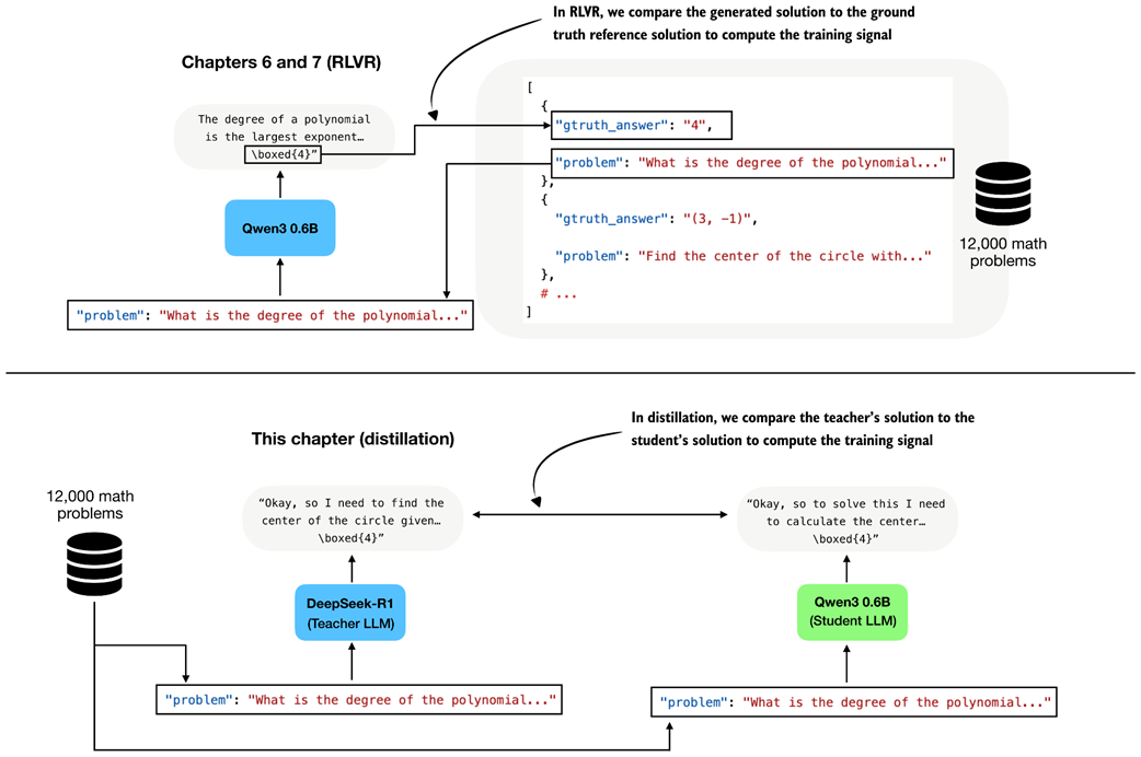 Figure 8.5 In RLVR, the generated answer is compared against the ground-truth reference solution (top subpanel), whereas in distillation the student answer is compared against the teacher-generated solution (bottom subpanel).
A practical advantage of distillation is that we can generate the teacher dataset ahead of time before training the student.
Because generating teacher answers for all 12,000 math problems can be time- and resource-intensive, I created this dataset ahead of time using the 671-billion-parameter DeepSeek-R1 model hosted via OpenRouter.
The full data generation cost was approximately $50 in API usage. Next, we simply load this pre-generated dataset, so you do not need to generate it yourself to follow along. If you are curious about the data-generation process, the code and usage instructions are available in the supplementary materials at https://github.com/rasbt/reasoning-from-scratch/tree/main/ch08/02_generate_distillation_data.
8.3 Loading the MATH training dataset for distillation
We now load the distilled MATH dataset generated by DeepSeek-R1 in the previous step. Each example contains a math problem together with a reasoning trace and final answer that we can use as the target for supervised fine-tuning. This step is highlighted in figure 8.6.
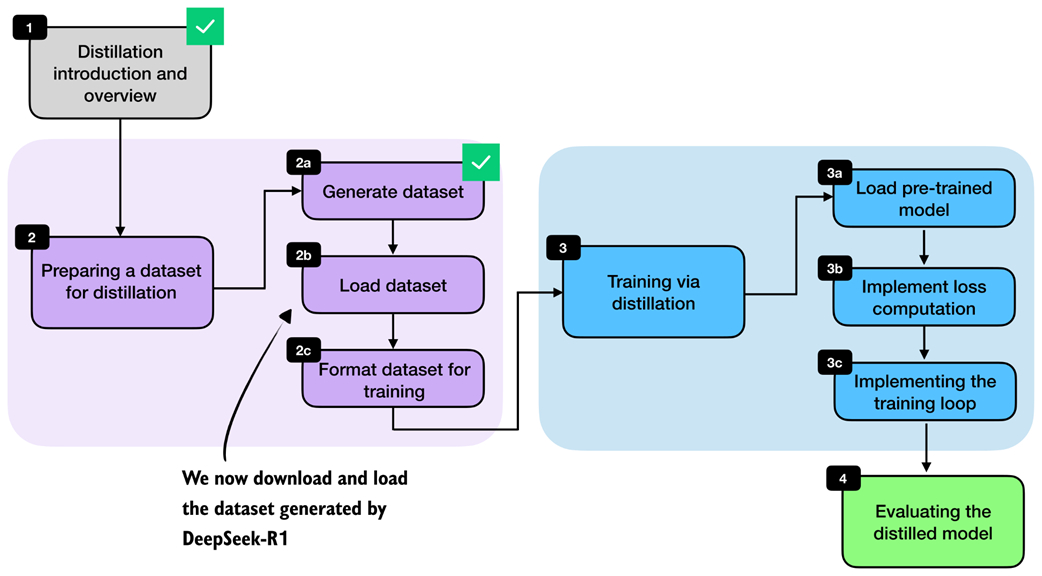 Figure 8.6 Chapter overview with the current section highlighted. Here, we load the DeepSeek-R1-generated dataset from a JSON file before preparing it for training.
I made the dataset available via the Hugging Face Hub, which is approximately 100 MB in size, at https://huggingface.co/datasets/rasbt/math_distill. The following helper function downloads the selected partition if it is not already cached locally and returns it as a Python object.
Listing 8.1 Loading the distilled MATH training split
import json
import requests
from pathlib import Path


def load_distill_data(
    local_path=None,
    partition="deepseek-r1-math-train",
    save_copy=True,
):

    if local_path is None:
        local_path = f"{partition}.json"
    local_path = Path(local_path)

    url = (
        "https://huggingface.co/datasets/rasbt/math_distill"
        "/resolve/main/data/"
        f"{partition}.json"
    )
    backup_url = (
        "https://f001.backblazeb2.com/file/reasoning-from-scratch/"
        f"MATH/{partition}.json"
    )

    if local_path.exists():
        # Reuse a cached copy if the dataset was already downloaded
        with local_path.open("r", encoding="utf-8") as f:
            data = json.load(f)

        size_kb = local_path.stat().st_size / 1e3
        print(f"{local_path}: {size_kb:.1f} KB (cached)")
        return data

    assert partition in (
        "deepseek-r1-math-train",
        "deepseek-r1-math500",
        "qwen3-235b-a22b-math-train",
        "qwen3-235b-a22b-math500",
    )

    try:
        # Try downloading from Hugging Face first
        r = requests.get(url, timeout=30)
        r.raise_for_status()
    except requests.RequestException:
        print("Using backup URL.")
        r = requests.get(backup_url, timeout=30)
        r.raise_for_status()

    data = r.json()

    if save_copy:
        # Save a local copy so later runs can skip the download
        with local_path.open("w", encoding="utf-8") as f:
            json.dump(data, f, indent=2)

        size_kb = local_path.stat().st_size / 1e3
        print(f"{local_path}: {size_kb:.1f} KB")

    return data
The output is:
deepseek-r1-math-train.json: 107538.0 KB
Dataset size: 12000
Next, let’s inspect one of the training examples to understand the dataset structure and see exactly what fields the teacher-generated data contains. For this, we pick one of the training examples (the fifth one) for illustration purposes:
from pprint import pprint
pprint(math_train[4])
The printed output is as follows:
{'gtruth_answer': '6',
 'message_content': 'Sam worked...'
 'message_thinking': "Okay, let's see. Sam was hired for 20 days...'
 'problem': 'Sam is hired for a 20-day period...'
}
Each dataset entry contains the math problem itself (problem), the ground-truth answer (gtruth_answer), the teacher’s reasoning trace in message_thinking, and the final answer in message_content.
For distillation, the two most important fields are the reasoning trace and the final answer, because together they form the target text that the student should learn to reproduce.
The format_distilled_answer function in listing 8.2 combines these two fields into a single training target by placing the reasoning trace inside <think>...</think> tags and then appending the final answer.
Listing 8.2 Formatting teacher responses for distillation
def format_distilled_answer(entry):
    content = str(entry["message_content"]).strip()
    if not content:
        raise ValueError("Missing non-empty 'message_content' field.")

    thinking = str(entry["message_thinking"]).strip()
    return f"<think>{thinking}</think>\n\n{content}"

print(format_distilled_answer(math_train[4]))
The printed output is:
<think>Okay, let's see. Sam was hired for 20 days. Each day he works, he earns $60...So answer is 6 days not worked.</think>
Sam worked \( x \) days and did not work \( y \) days. We know:...
Sam did not work \(\boxed{6}\) days.
As discussed in the previous chapter, the <think></think> tokens are optional. They are not required for distillation itself, though they can be useful for clearly separating the reasoning trace from the final answer.
This separation becomes helpful when implementing user interfaces that hide the verbose reasoning trace from end users. Some systems, including products such as ChatGPT, may display only the final answer while hiding portions of the internal reasoning. Teaching the model to use explicit <think> tags makes these traces easier to parse and handle.
Since the dataset also contains ground-truth labels, we can measure how accurate the teacher model was on this set. For convenience, we use the evaluate_json.py script from the supplementary materials of chapter 3, which compares generated answers against the reference answers using the verifier implemented in that chapter. This gives us a quick estimate of DeepSeek-R1’s performance on the distillation dataset.
from reasoning_from_scratch.ch07 import download_from_github
_ = download_from_github(
    "ch03/02_math500-verifier-scripts/evaluate_json.py"
)
After downloading the script via the preceding Python code, we can run it in a code terminal as follows:
uv run evaluate_json.py \
--json_path "deepseek-r1-math-train.json" \
--gtruth_answer gtruth_answer \
--generated_text message_content
(If you are not a uv user, replace uv run with python.)
The output is:
Accuracy: 90.6% (10871/12000)
While the model is not perfect, 90.6% is a relatively high accuracy. Furthermore, on the MATH-500 test set from chapter 3, it achieved 91.2% accuracy, which is much higher than the Qwen3 0.6B base model we are going to train (15.2% accuracy on MATH-500) or the official Qwen3 0.6B reasoning reference model (50.8% on MATH-500).
8.4 Building training examples
Next, we convert the raw dataset entries into training examples that can be consumed by the model. At a high level, this means formatting the prompts and answers consistently, tokenizing them, and storing the resulting token IDs together with the prompt length. The overall preprocessing stage is highlighted in figure 8.7.
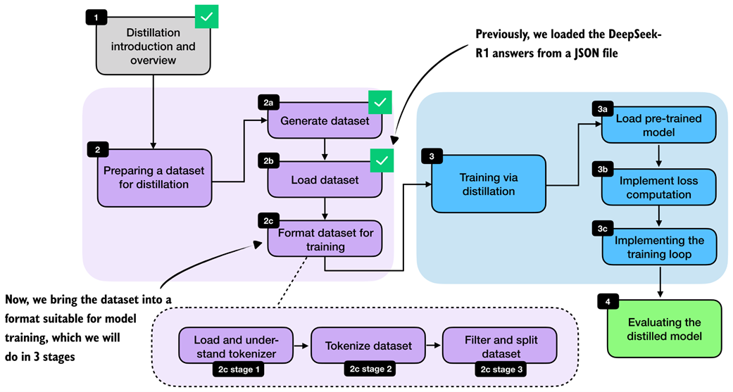 Figure 8.7 Bringing the loaded dataset into a format suitable for model training by understanding the tokenizer, tokenizing the examples, and filtering and splitting the dataset.
Most of the work here is straightforward preprocessing. In the RLVR chapters, we performed similar preparation on the fly because each training example was sampled once and then discarded. Distillation is different, and we usually loop over the same examples for multiple training epochs. It is therefore more efficient to format and tokenize the dataset once, store the processed examples, and reuse them during training. This is also one reason distillation is often easier to iterate on than RLVR once the teacher data has been collected.
What are training epochs? Training epoch, or epoch for short, is a classical machine learning and deep learning term. An epoch is one complete pass through the full training dataset. For example, if we train for three epochs, the model sees each training example three times, usually in a different order each time. Multiple epochs help the model gradually improve by revisiting the same data more than once.
8.4.1 Loading and understanding the tokenizer
We begin with the tokenizer. Here, we use the Qwen3 reasoning tokenizer because it supports the <think>...</think> tokens introduced in chapter 7.
Listing 8.3 Loading the Qwen3 reasoning tokenizer
from reasoning_from_scratch.qwen3 import (
    download_qwen3_small,
    Qwen3Tokenizer,
)


def load_reasoning_tokenizer(local_dir="qwen3"):
    download_qwen3_small(
        kind="reasoning", tokenizer_only=True, out_dir=local_dir
    )

    tokenizer_path = Path(local_dir) / "tokenizer-reasoning.json"
    tokenizer = Qwen3Tokenizer(
        tokenizer_file_path=tokenizer_path,
        apply_chat_template=True,
        add_generation_prompt=True,
        add_thinking=True,
    )

    return tokenizer

tokenizer = load_reasoning_tokenizer()
We set apply_chat_template=True and add_generation_prompt=True so that the tokenizer applies the same style of prompt formatting used by Qwen3’s chat and reasoning models. The example below shows the additional wrapper tokens that are inserted automatically.
prompt = "Sam is hired for a 20-day period..."
prompt_ids = tokenizer.encode(prompt)
decoded_prompt = tokenizer.decode(prompt_ids)
print(decoded_prompt)
The formatted text is as follows:
<|im_start|>user
Sam is hired for a 20-day period...<|im_end|>
<|im_start|>assistant
In particular, <|im_start|>user marks the start of the user prompt, <|im_end|> marks the end of the prompt, and <|im_start|>assistant marks the start of the model response. This chat-style wrapping is optional, but it is a common convention for instruction and chat fine-tuning.
For the target answer, we disable this wrapping by setting chat_wrapped=False. Otherwise, both the prompt and the answer would introduce their own assistant-start tokens, which is not what we want when concatenating them into a single training sequence:
answer = (
    "<think>Okay, let me try to solve "
    "this problem...</think> \\boxed{4}"
)
answer_ids = tokenizer.encode(answer, chat_wrapped=False)
decoded_answer = tokenizer.decode(answer_ids)
print(decoded_answer)
As shown, the chat_wrapped=False setting suppresses the chat template for the answer tokens:
<think>Okay, let me try to solve this problem...</think> \boxed{4}
For training, we need the full sequence of token IDs: the wrapped prompt, followed by the teacher answer, followed by an end-of-sequence token. This is the sequence the model will see during next-token prediction:
token_ids = prompt_ids + answer_ids + [tokenizer.eos_token_id]
decoded_token_ids = tokenizer.decode(token_ids)
print(decoded_token_ids)
The formatted string looks like as follows:
<|im_start|>user
Sam is hired for a 20-day period...<|im_end|>
<|im_start|>assistant
<think>Okay, let me try to solve this problem...</think>\boxed{4}<|im_end|>
It is worth emphasizing that the reasoning tokenizer is mainly convenient because it already includes the <think></think> tokens. But in principle, we could also use the base tokenizer. Likewise, the chat template is not strictly required. We keep it here because it matches the formatting used by Qwen3’s own reasoning models and helps keep the training and evaluation setup consistent.
If you later evaluate the model with the scripts from earlier chapters, remember to use the --which_model "reasoning" setting so that the evaluation uses the same tokenizer variant.
8.4.2 Formatting and tokenizing the dataset
After loading and understanding the tokenizer, we can now apply the formatting and tokenization steps to the whole dataset. This transition is highlighted in figure 8.8.
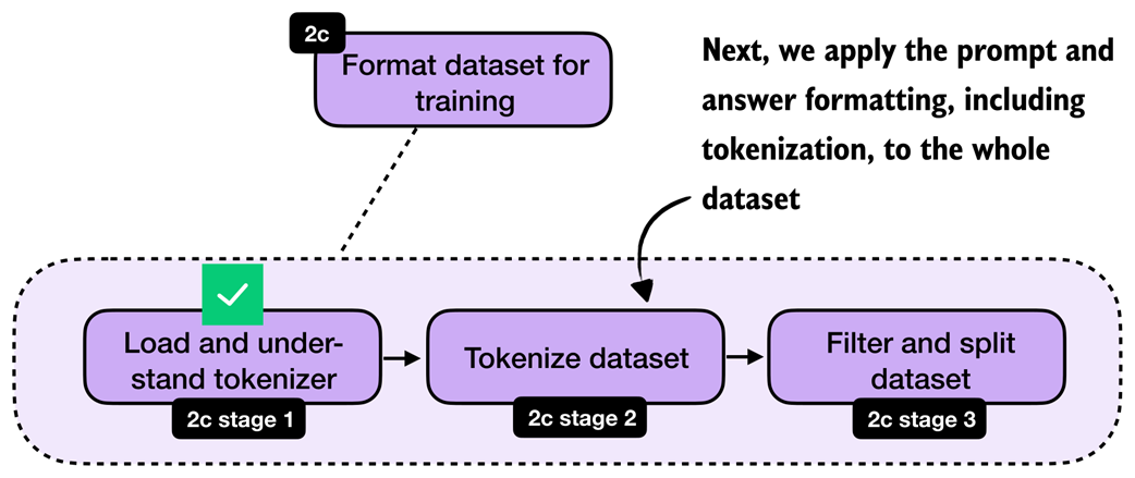 Figure 8.8 With the tokenizer step complete, we now move on to apply the formatting and tokenization steps to the whole dataset.
With the tokenizer in place, we can now apply the formatting and tokenization steps consistently across the whole dataset via a build_examples function. The full formatting and tokenization pipeline for a single training sample is illustrated in figure 8.9.
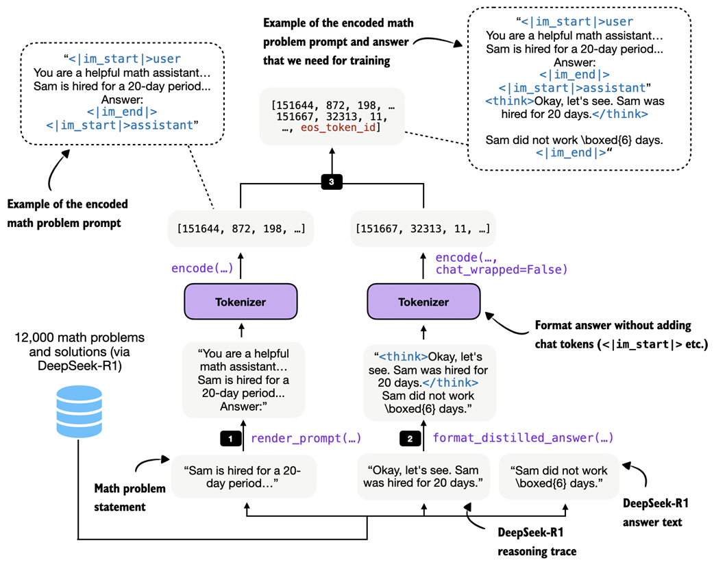 Figure 8.9 Example of the tokenization pipeline for one training sample. The math problem is rendered into the chat prompt format, the teacher reasoning trace and final answer are combined via
 format_distilled_answer, and both parts are concatenated into one token sequence.
As shown in figure 8.9, the build_examples function follows three steps. First, it renders and tokenizes the prompt. Second, it formats and tokenizes the teacher answer. Third, it concatenates both parts and records the prompt length so that we can later compute the loss only on the answer tokens. Listing 8.4 shows how to implement that in code.
Listing 8.4 Building and inspecting tokenized distillation examples
from reasoning_from_scratch.ch03 import render_prompt


def build_examples(data, tokenizer):
    examples = []
    skipped = 0

    for entry in data:
        try:
            # Step 1: Render the problem in the chat format
            prompt = render_prompt(entry["problem"])
            prompt_ids = tokenizer.encode(prompt)

            # Step 2: Tokenize the teacher reasoning trace and final answer
            target_answer = format_distilled_answer(entry)
            answer_ids = tokenizer.encode(
                target_answer, chat_wrapped=False
            )

            # Step 3: Combine prompt and answer for training
            token_ids = (
                prompt_ids + answer_ids + [tokenizer.eos_token_id]
            )

            if len(token_ids) < 2:
                skipped += 1
                continue

            # Store prompt length so we can ignore prompt tokens in the loss later
            examples.append({
                "token_ids": token_ids,
                "prompt_len": len(prompt_ids),
            })
        except (KeyError, TypeError, ValueError):
            # Skip misformatted examples
            skipped += 1

    return examples, skipped


examples, skipped = build_examples(math_train, tokenizer)

print("Number of examples:", len(examples))
print("Number of skipped examples:", skipped)
The resulting numbers, after running the code in listing 8.4, are:
Number of examples: 12000
Number of skipped examples: 0
Next, let’s decode one of the training examples to inspect it further:
print(tokenizer.decode(examples[4]["token_ids"]))
The output is:
<|im_start|>user
You are a helpful math assistant.
Answer the question and write the final result on a new line as:
\boxed{ANSWER}

Question:
Sam is hired for a 20-day period...

Answer:<|im_end|>
<|im_start|>assistant
<think>Okay, let's see. Sam was hired for 20 days.... So answer is 6 days not worked.</think>
...Sam did not work \(\boxed{6}\) days.<|im_end|>
Looking at the output above, we can confirm that it checks all the formatting requirements. For instance, it uses the chat template correctly, and the answer’s reasoning trace is correctly enclosed in <think></think> tags. Finally, the answer ends with an end-of-sequence token, <|im_end|>.
8.4.3 Filtering and splitting the dataset
Once the examples are tokenized, we still need to filter long sequences and split the dataset into training and validation subsets. This step is highlighted in figure 8.10.
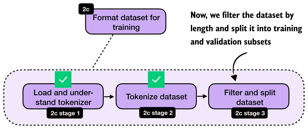 Figure 8.10 After tokenization, we filter out long sequences and split the remaining examples into training and validation subsets.
After tokenization, it is useful to inspect the sequence lengths. This tells us how long the examples are on average, which samples are extreme outliers, and how aggressive our filtering needs to be. We then remove examples above the chosen maximum length, shuffle the remaining data with a fixed random seed, and split off a small validation set.
Let’s begin with analyzing the sequence lengths via listing 8.5.
Listing 8.5 Computing lengths and filtering long examples
def compute_length(examples, answer_only=False):
    lengths = []
    for ex in examples:
        total = len(ex["token_ids"])
        length = total - ex["prompt_len"] if answer_only else total
        lengths.append(length)

    avg_len = round(sum(lengths) / len(lengths))

    shortest_len = min(lengths)
    longest_len = max(lengths)
    shortest_idx = lengths.index(shortest_len)
    longest_idx = lengths.index(longest_len)

    print(f"Average: {avg_len} tokens")
    print(f"Shortest: {shortest_len} tokens (index {shortest_idx})")
    print(f"Longest: {longest_len} tokens (index {longest_idx})")

compute_length(examples)
The resulting output is:
Average: 2946 tokens
Shortest: 236 tokens (index 10846)
Longest: 42005 tokens (index 2529)
As we can see, the average response length is at 2,946 tokens, which is typical for reasoning models. There are outliers, though. For instance, the longest answer is 42,005 tokens, which is very excessive. The index positions (index 10846 and index 2529) denote the positions of the shortest and longest examples in the dataset, respectively, in case we want to inspect them.
To keep the computational costs reasonable for this distillation example, we filter the dataset to include only dataset entries of up to 2,048 tokens, using the code in listing 8.6. In practice, controlling the sequence length is one of the main steps that makes distillation feasible on smaller hardware.
Listing 8.6 Filtering long examples
def filter_examples_by_max_len(examples, max_len=2048):
    filtered_examples = [
        s for s in examples
        if len(s["token_ids"]) <= max_len
    ]

    print("Original:", len(examples))
    print("Filtered:", len(filtered_examples))
    print("Removed:", len(examples) - len(filtered_examples))

    return filtered_examples


filtered_examples = filter_examples_by_max_len(examples, max_len=2048)
After running the filtering code in listing 8.6, 5305 training examples were removed:
Original: 12000
Filtered: 6695
Removed: 5305
Let’s compute the dataset lengths on this new subset:
compute_length(filtered_examples)
As we can see, the average token length is now down to 1180 tokens, and none of the formatted training examples exceed the 2048 tokens.
Average: 1180 tokens
Shortest: 236 tokens (index 5971)
Longest: 2048 tokens (index 5587)
Lastly, we split the dataset into training and validation examples, where the latter are used for quick evaluations throughout the training run later.
Listing 8.7 Partitioning into training and validation sets
import random

rng = random.Random(123)
rng.shuffle(filtered_examples)

train_examples = filtered_examples[25:]
val_examples = filtered_examples[:25]

print("Number of train examples:", len(train_examples))
print("Number of validation examples:", len(val_examples))
The resulting numbers of training and validation examples are as follows:
Number of train examples: 6670
Number of validation examples: 25
Note that we keep the validation set purposefully small so that we don’t unnecessarily slow down the training loop. In addition, after the training is completed, we will also use the 500 samples of the MATH-500 set to evaluate the performance of the model.
Exercise 8.1: Training and validation set lengths Apply the
compute_lengthfunction to the newtrain_examplesandval_examplespartitions to check whether they are balanced based on the sample lengths.
8.5 Loading a pre-trained model
With the dataset preparation complete, we can turn to the actual distillation training. We begin by loading the pre-trained Qwen3 base model, as shown in figure 8.11.
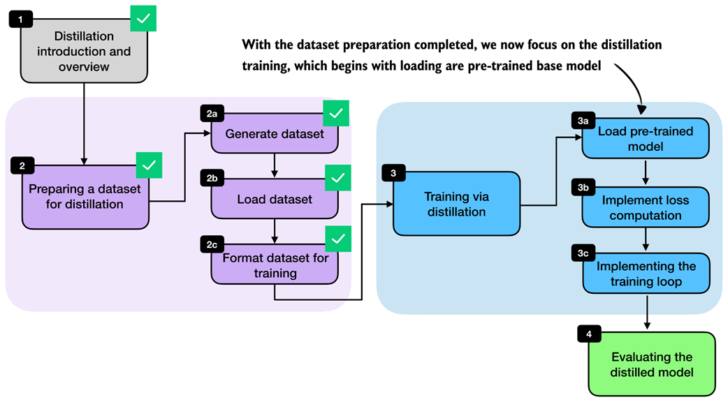 Figure 8.11 With the dataset preparation complete, we begin the distillation training by loading the pre-trained Qwen3 base model.
We start from the pre-trained Qwen3 base model, not from an RL-trained model, because distillation itself is the training stage we want to study here. This keeps the setup clean and makes it easier to attribute any improvement to the distilled reasoning traces. It also mirrors a common practical setup where a general base model is adapted later using teacher-generated data.
Listing 8.8 Loading the Qwen3 base model for distillation
import torch

from reasoning_from_scratch.ch02 import get_device
from reasoning_from_scratch.ch03 import (
    load_model_and_tokenizer,
)

device = get_device()

model, _ = load_model_and_tokenizer(
    which_model="base",
    device=device,
    use_compile=False,
)
Note that we can ignore the loaded base tokenizer in listing 8.8, since we will be using the tokenizer with <think></think> token support we loaded previously in section 8.4.1.
8.6 Computing the training and validation losses
Next, we implement the cross-entropy loss that serves as the training signal during distillation when we implement the training loop later. We will also reuse the same computation on the validation set to monitor progress during training.
Readers with a deep-learning background may already know cross-entropy from classification tasks. The idea is the same here, except that the target class we want to predict at each position is the next token in the teacher-generated sequence.
We can connect this loss directly to the log-probability computations from chapters 5 and 6. As discussed there, log-probability measures how much probability the model assigns to the correct next token. Higher log-probability means the model is more confident in the correct token, and lower log-probability means the opposite. Re-using the “The capital of Germany is Berlin” example from previous chapters, this is recapped in figure 8.12.
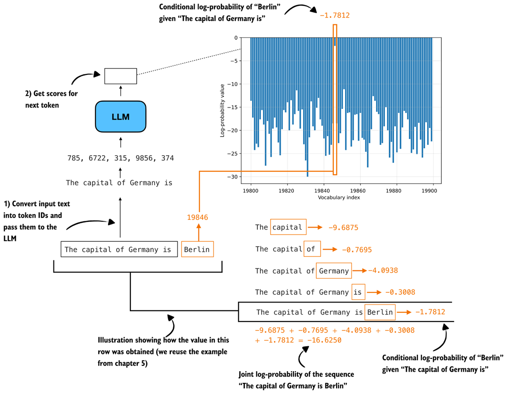 Figure 8.12 Illustration of token and sequence log-probabilities. The log-probabilities of the correct next tokens are summed to obtain the sequence log-probability, which is the basis for the cross-entropy loss used later in this chapter.
Cross-entropy is simply the negative average of these token log-probabilities shown in figure 8.12. For instance, if -16.6250 is the log-probability, the negative log-probability is 16.6250, the negative average log-probability is 16.6250/5 = 3.325. Note that the 5 is there because the sequence has 5 target predictions whose log-probabilities are being averaged.
The cross-entropy is also 3.325. (Similar to log-probability, the closer the value is to 0, the better, since the model is more confident in the correct target token.)
The sequence_logprob function from chapter 6 performs exactly this computation shown in figure 8.12, which makes it a useful starting point for understanding how the distillation loss works. In this case, we use the training example at index position 5730, because it’s the shortest example in train_examples, which we can determine via compute_length(train_examples), and thus computes a bit more quickly than the other examples:
token_ids = train_examples[5730]["token_ids"]
prompt_len = train_examples[5730]["prompt_len"]
Instead of reporting the summed log-probabilities returned by sequence_logprob, we average them over the number of answer tokens. The reason is that summed log-probabilities grow with sequence length, so they are not directly comparable across examples with shorter or longer answers. By dividing by the number of answer tokens, we obtain a per-token quantity, which matches the form used by cross-entropy loss. We compute the number of answer tokens by subtracting prompt_len from the total sequence length:
Listing 8.9 Computing average negative log-probabilities
from reasoning_from_scratch.ch06 import sequence_logprob

tok = torch.tensor(token_ids, dtype=torch.long, device=device)

with torch.no_grad():
    seq_logprob = sequence_logprob(model, tok, prompt_len)
    num_answer_tokens = tok.numel() - prompt_len
    avg_logprob = -seq_logprob / num_answer_tokens
print(f"Average logprob: {avg_logprob:.2f}")
The resulting negative average log-probability is 1.68.
Now, we can compute the same quantity using PyTorch’s cross_entropy function. Although the function is usually introduced for classification, it is a natural choice here. For instance, the model logits provide the predicted class distribution over the vocabulary, and the target sequence provides the correct class label at each position.
As in the previous average-logprob calculation, we compute the loss only over the answer tokens and ignore the prompt tokens (the prompt is the context provided as input, and it is not something we want the model to be penalized for reproducing). This is illustrated in figure 8.13.
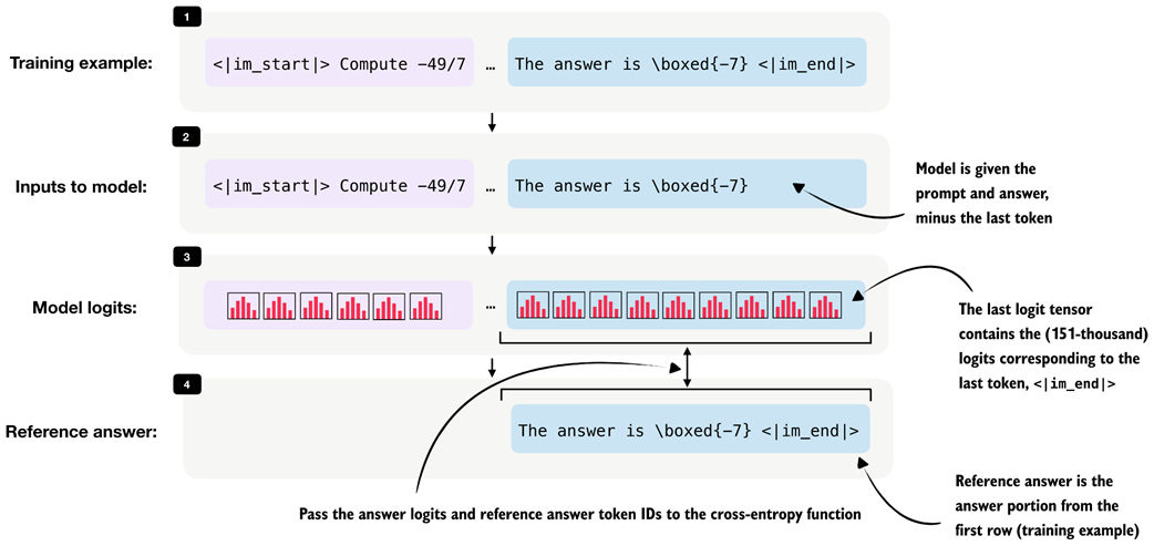 Figure 8.13 Illustration of the input for the cross-entropy loss over the answer tokens. The model receives the prompt and answer shifted by one token as input, and the answer-token logits are compared against the reference answer tokens.
During distillation, we want the student to learn the teacher’s reasoning trace and final answer conditioned on the prompt, so, as shown in figure 8.13, we discard the logits and targets that correspond only to the prompt portion of the sequence when computing the cross-entropy in listing 8.10:
Listing 8.10 Computing cross-entropy loss directly
# Shift the sequence by one token so each input predicts the next token target
input_ids = tok[:-1].unsqueeze(0)
target_ids = tok[1:]
logits = model(input_ids).squeeze(0)

# Drop the prompt positions so the loss only covers the teacher answer
first_answer_logit_idx = max(prompt_len - 1, 0)
answer_logits = logits[first_answer_logit_idx:]
answer_targets = target_ids[first_answer_logit_idx:]

# Compute cross-entropy loss
with torch.no_grad():
    ce_mean_direct = torch.nn.functional.cross_entropy(
        answer_logits, answer_targets
    )
print(f"Cross-entropy: {ce_mean_direct:.2f}")
The resulting cross-entropy loss is 1.68, which is similar to listing 8.9, when we used the sequence_logprob function. In other words, cross_entropy is implementing the same core calculation in a more optimized way. For training, we therefore use the built-in cross_entropy function rather than our custom log-probability function.
The compute_example_loss helper in listing 8.11 below wraps this logic into a convenient function that calculates the answer-only loss for a single example. “Answer-only loss” means the training loss is computed only on the teacher’s answer tokens, not on the prompt tokens.
We focus on the answer-only loss because the prompt is already given. And the model’s job in distillation is not to learn to reconstruct the input instruction. Its job is to produce the target answer conditioned on that instruction. So we use the prompt as context, but we do not penalize the model for prompt-token predictions.
Now, let’s put it all together into a function that applies the whole logic, from target preparation to cross entropy computation, on a given training example in listing 8.11:
Listing 8.11 Defining the loss for one distillation example
def compute_example_loss(model, example, device):
    token_ids = example["token_ids"]
    prompt_len = example["prompt_len"]

    # Create input-target pairs that are shifted by one token
    input_ids = torch.tensor(
        token_ids[:-1], dtype=torch.long, device=device
    ).unsqueeze(0)
    target_ids = torch.tensor(
        token_ids[1:], dtype=torch.long, device=device
    )

    logits = model(input_ids).squeeze(0)

    # Ignore prompt tokens so the loss is computed on the distilled answer only
    answer_start = max(prompt_len - 1, 0)
    answer_logits = logits[answer_start:]
    answer_targets = target_ids[answer_start:]

    # Compute cross-entropy loss
    loss = torch.nn.functional.cross_entropy(
        answer_logits, answer_targets
    )
    return loss

# Use to verify that the helper returns the same loss as before
with torch.no_grad():
    loss = compute_example_loss(
        model, train_examples[5730], device
    )

print(f"Loss: {loss:.2f}")
The resulting loss is 1.68 again, which indicates that the function in listing 8.11 works as intended.
Batching It is also possible to process multiple examples in parallel by batching them together. We omit batching here to keep the implementation compact and the resource requirements lower. Appendix E discusses batching and throughput-oriented execution in more detail for the loss computation and training in general.
Next, we define a small wrapper that iteratively computes the average loss across multiple examples. This will be useful both for quick sanity checks and for tracking the validation loss during training.
Listing 8.12 Evaluating loss across multiple examples
@torch.no_grad()
def evaluate_examples(model, examples, device):
    was_training = model.training

    # Temporarily switch to evaluation mode while scoring the examples
    model.eval()
    total_loss = 0.0
    num_examples = 0

    # Sum the loss over all examples
    for example in examples:
        loss = compute_example_loss(model, example, device)
        total_loss += loss.item()
        num_examples += 1

    # Restore training mode so this helper is safe to call during training
    if was_training:
        model.train()

    # Average the loss over all examples
    return total_loss / num_examples

# Estimate the current training loss on a small subset
train_loss = evaluate_examples(model, train_examples[:3], device)
print(f"Train loss (3 examples): {train_loss:.2f}")

val_loss = evaluate_examples(model, val_examples[:3], device)
print(f"Validation loss (3 examples): {val_loss:.2f}")
The output is:
Train loss (3 examples): 0.98
Validation loss (3 examples): 1.02
We will reuse this evaluation function during training. Ideally, both quantities should decrease over time, which indicates that the student model is becoming better at matching the teacher-generated target sequences.
In practice, the training loss, which is the loss computed on the training examples used for optimization, is often noisy because it is measured on the examples currently being optimized and can fluctuate depending on the sample order and recent parameter updates.
The validation loss, which is measured on a separate hold-out validation set rather than on the examples currently being used for optimization, is computed without updating the model weights. As a result, it usually provides a cleaner signal of whether the student is improving in a way that generalizes beyond the training set. For this reason, the validation loss is often the more reliable metric to watch.
8.7 Implementing the training loop for distillation
With the dataset preparation and loss computation in place, we can now implement the training loop for distillation. This stage is highlighted in figure 8.14.
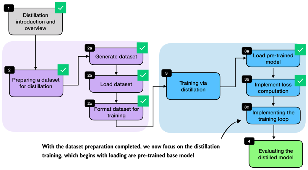 Figure 8.14 With dataset preparation and loss computation complete, we now turn to the training loop for distillation.
The training loop is very similar to the one from chapter 6. The main difference is that we now revisit the same training set multiple times across epochs and optimize the cross-entropy distillation loss instead of the reinforcement learning objective used in RLVR. The detailed steps are shown in figure 8.15.
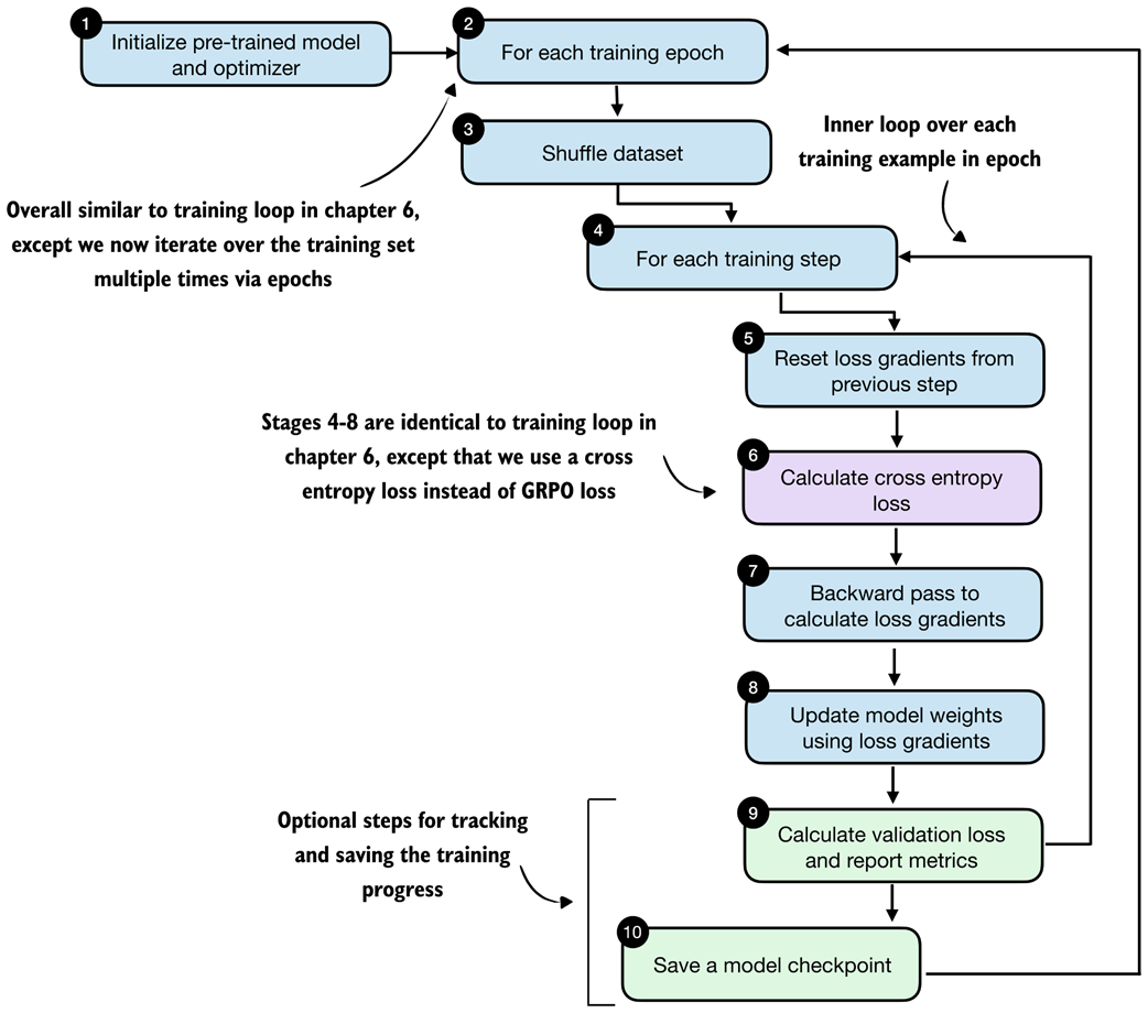 Figure 8.15 Distillation training loop. In each epoch, the training examples are shuffled, the student model computes a cross-entropy loss for each example, gradients are backpropagated, and the model weights are updated. The validation loss is reported in certain intervals to track progress.
The train_distillation function in listing 8.13 implements the loop shown in figure 8.15. It shuffles the training examples at the start of each epoch, computes the loss for each example, applies an optimizer step, optionally clips large gradients, and periodically evaluates on the validation set. The metrics are also written to a CSV file so that we can inspect the learning curves later.
Listing 8.13 Implementing the distillation training loop
import time


def train_distillation(
    model,
    train_examples,
    val_examples,
    device,
    epochs=2,
    lr=5e-6,
    grad_clip_norm=None,
    seed=123,
    log_every=50,
    checkpoint_dir="checkpoints",
    csv_log_path=None,
):
    # Step 1: initialize optimizer (model is already loaded)
    optimizer = torch.optim.AdamW(model.parameters(), lr=lr)
    model.train()

    total_steps = epochs * len(train_examples)
    global_step = 0
    rng = random.Random(seed)

    if csv_log_path is None:
        timestamp = time.strftime("%Y%m%d_%H%M%S")
        csv_log_path = f"train_distill_metrics_{timestamp}.csv"
    csv_log_path = Path(csv_log_path)

    # Step 2: iterate over training epochs
    for epoch in range(1, epochs + 1):
        # Step 3: shuffle the training examples at the start of the epoch
        epoch_examples = list(train_examples)
        rng.shuffle(epoch_examples)

        # Step 4: iterate over training examples in epoch
        for example in epoch_examples:
            global_step += 1

            # Stage 5: reset loss gradient
            optimizer.zero_grad()

            # Step 6: compute the cross-entropy loss for the current example
            loss = compute_example_loss(model, example, device)

            # Step 7: backpropagate gradients
            loss.backward()

            # Optionally clip large gradients to improve training stability
            if grad_clip_norm is not None:
                torch.nn.utils.clip_grad_norm_(
                    model.parameters(), grad_clip_norm
                )

            # Step 8: update the model weights
            optimizer.step()

            # Step 9: periodically evaluate the current model on the validation set
            if log_every and global_step % log_every == 0:
                val_loss = evaluate_examples(
                    model=model,
                    examples=val_examples,
                    device=device,
                )
                model.train()
                print(
                    f"[Epoch {epoch}/{epochs} "
                    f"Step {global_step}/{total_steps}] "
                    f"train_loss={loss.item():.4f} "
                    f"val_loss={val_loss:.4f}"
                )
                append_csv_metrics(
                    csv_log_path=csv_log_path,
                    epoch_idx=epoch,
                    total_steps=global_step,
                    train_loss=loss.item(),
                    val_loss=val_loss,
                )

        # Step 10: record the metrics and save a checkpoint for this epoch
        ckpt_path = save_checkpoint(
            model=model,
            checkpoint_dir=checkpoint_dir,
            step=global_step,
            suffix=f"epoch{epoch}",
        )
        print(f"Saved checkpoint to {ckpt_path}")
    return model


def save_checkpoint(model, checkpoint_dir, step, suffix=""):
    checkpoint_dir = Path(checkpoint_dir)
    checkpoint_dir.mkdir(parents=True, exist_ok=True)
    suffix = f"-{suffix}" if suffix else ""
    ckpt_path = (
        checkpoint_dir /
        f"qwen3-0.6B-distill-step{step:05d}{suffix}.pth"
    )
    torch.save(model.state_dict(), ckpt_path)
    return ckpt_path


def append_csv_metrics(
    csv_log_path,
    epoch_idx,
    total_steps,
    train_loss,
    val_loss,
):
    if not csv_log_path.exists():
        csv_log_path.write_text(
            "epoch,total_steps,train_loss,val_loss\n",
            encoding="utf-8",
        )
    with csv_log_path.open("a", encoding="utf-8") as f:
        f.write(
            f"{epoch_idx},{total_steps},{train_loss:.6f},"
            f"{val_loss:.6f}\n"
        )
With a maximum sequence length of 2048, the full training run requires about 15 GB of VRAM memory. If this is too high for your hardware, you can lower the resource requirements by filtering out longer sequences earlier in the notebook, for example by changing max_len from 2048 to 1024 or 512 in the filter_examples_by_max_len step in listing 8.6 (section 8.4.3).
Let’s execute a short training run:
Listing 8.14 Training the model
# Seed PyTorch so the short demo is reproducible
torch.manual_seed(0)

# Train on a tiny subset so this notebook run stays lightweight
train_distillation(
    model,
    train_examples=train_examples[:10],
    val_examples=val_examples[:10],
    device=device,
    epochs=2,
    lr=5e-6,
    grad_clip_norm=1.0,
    seed=123,
    log_every=5,
    # Same as in chapter 6
    csv_log_path="train_distill_metrics.csv",
)
Let’s briefly go over the settings before we inspect the results. We keep the training run intentionally short. For instance, we use only the first 10 training examples and 10 validation examples, and we train for just 2 epochs. This is purely to keep the notebook run lightweight and fast enough for experimentation. For a real distillation run, we would of course train on many more examples, ideally the whole training set.
The learning rate (lr=5e-6) is in a reasonable range for fine-tuning a pre-trained model and works well in practice for this setup and worked well in practice in my experiments, as reflected in the loss curves discussed next.
The gradient clipping setting (grad_clip_norm=1.0) is the same as in chapter 6 and helps prevent unstable updates when a particular example produces unusually large gradients.
The log_every=5 setting means that validation loss is measured every 5 training steps. Since this demo uses only a handful of examples, this produces frequent progress updates so that we can quickly verify that the training loop behaves as expected. In a larger run, we would usually increase this interval to reduce evaluation overhead.
Finally, the csv_log_path="train_distill_metrics.csv" argument stores the training and validation losses in a CSV file so that we can inspect and plot them later.
The main goal of this run is not to achieve the best possible reasoning performance, but to confirm that the distillation pipeline works end to end. Once that is established, we can move on to larger runs and inspect the resulting learning curves and checkpoints in more detail.
Let’s now take a brief look at the run’s output:
[Epoch 1/2 Step 5/20] train_loss=0.9648 val_loss=0.9082
[Epoch 1/2 Step 10/20] train_loss=0.9844 val_loss=0.8871
Saved checkpoint to checkpoints/qwen3-0.6B-distill-step00010-epoch1.pth
[Epoch 2/2 Step 15/20] train_loss=0.8008 val_loss=0.8707
[Epoch 2/2 Step 20/20] train_loss=0.7148 val_loss=0.8586
Saved checkpoint to checkpoints/qwen3-0.6B-distill-step00020-epoch2.pth
Even though this is only a tiny demonstration run, the output already shows the expected overall behavior. Both the training loss and the validation loss decrease over time, which indicates that the student model is becoming better at matching the teacher-generated target sequences. The validation loss is especially useful here because it is computed on hold-out examples and therefore provides a cleaner signal that the improvement is not limited to the training samples alone.
We can also see that checkpoints are saved at the end of each epoch. This is useful in practice because it allows us to resume training later or evaluate intermediate versions of the distilled model using the MATH-500 test set.
8.8 Evaluating the distilled model
After implementing the training loop, the final stage is evaluation of the distilled model, as shown in figure 8.16.
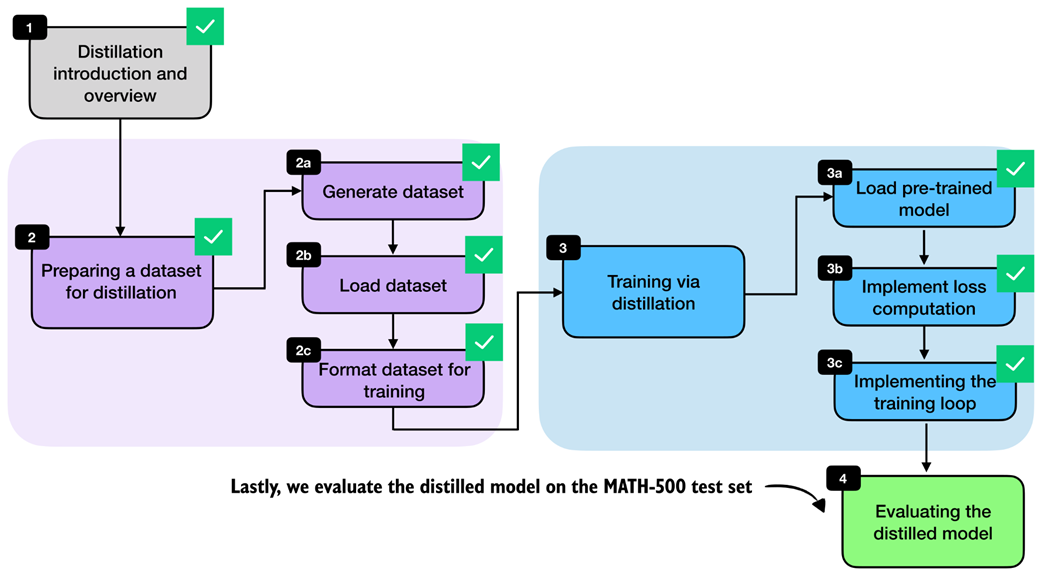 Figure 8.16 After implementing the training loop, we evaluate the distilled model on the MATH-500 test set.
Instead of running the full distillation process inside this notebook, we can also download a convenience script from the supplementary materials. As in the previous chapter on RLVR, it is often convenient to keep the notebook focused on the core ideas and move the longer-running training logic into a standalone script.
from reasoning_from_scratch.ch07 import download_from_github
download_from_github(
    "ch08/04_train_with_distillation/distill.py"
)
After downloading the script via the preceding code, we can run it as follows in a code terminal (if you are not a uv user, replace uv run with python):
uv run distill.py \
--data_path deepseek-r1-math-train.json \
--validation_size 25 \
--epochs 3 \
--lr 1e-5 \
--max_seq_len 2048 \
--use_think_tokens \
--grad_clip 1.0
Using these settings, the full training run takes about 3 hours and 5 minutes on a GPU System and uses roughly 15.02 GB of GPU memory. (This is relatively modest compared with the earlier RLVR runs because most of the expensive work has already been moved into the one-time teacher data generation step.) If you do not want to run the training yourself, we can download the resulting metrics file and inspect it directly.
download_from_github(
    "ch08/03_logs/deepseek-r1-2048_distill_metrics.csv"
)
The following listing 8.15 implements a utility function to visualize the training metrics stored in the CSV file:
Listing 8.15 Plotting distillation losses from a CSV log
import csv
import matplotlib.pyplot as plt


def plot_distill_metrics(csv_path="train_distill_metrics.csv"):
    total_steps, train_losses, val_losses, epoch_bounds = [], [], [], {}

    # Load and plot the logged losses
    with open(csv_path, newline="", encoding="utf-8") as f:
        for row in csv.DictReader(f):
            step = int(row["total_steps"])
            epoch = int(row["epoch"])
            total_steps.append(step)
            train_losses.append(float(row["train_loss"]))
            val_losses.append(float(row["val_loss"]))
            epoch_bounds.setdefault(epoch, [step, step])[1] = step

    fig, ax = plt.subplots(figsize=(7, 4))
    ax.plot(total_steps, train_losses, label="train_loss", alpha=0.3)
    ax.plot(total_steps, val_losses, label="val_loss")
    ax.set_xlabel("Total Steps")
    ax.set_ylabel("Loss")
    ax.legend()

    # Add a second x-axis so the epoch numbers are visible below the step axis
    epoch_axis = ax.secondary_xaxis("bottom")
    epoch_axis.spines["bottom"].set_position(("outward", 45))
    epochs = sorted(epoch_bounds)
    epoch_axis.set_xticks(
        [
            (epoch_bounds[epoch][0] + epoch_bounds[epoch][1]) / 2
            for epoch in epochs
        ]
    )
    epoch_axis.set_xticklabels(epochs)
    epoch_axis.set_xlabel("Epoch")

    plt.tight_layout()
    plt.show()


plot_distill_metrics("deepseek-r1-2048_distill_metrics.csv")
The resulting plot is shown in figure 8.17.
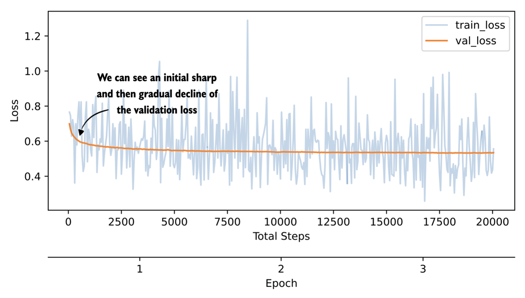 Figure 8.17 Plot showing the training and validation loss of a 3-epoch distillation training run on DeepSeek-R1 reasoning traces.
The training-loss curve and validation-loss curve shown in figure 8.17 should be interpreted slightly differently. The training loss is computed for each training example during training at the current step, whereas the validation loss is computed on a small fixed hold-out set. The validation curve is therefore less noisy and the more informative signal here. We could also compute the training loss on a subset of examples, similar to the validation loss, but this would slow down the training; the training loss is much less important than the validation loss for estimating the training progress.
As we would hope, the validation loss drops sharply at first and then begins to flatten out, indicating that the model is learning from the distillation data but that additional training yields diminishing returns. We could experiment with a larger learning rate or a different schedule to train more aggressively, but overall the curve looks healthy.
Just as in chapter 7, we can evaluate saved checkpoints with the verifier-based utilities from chapter 3. The following command downloads the evaluation script from the supplementary materials:
download_from_github(
    "ch03/02_math500-verifier-scripts/evaluate_math500.py"
)
Next, we evaluate the distilled checkpoint on MATH-500 using the reasoning tokenizer in a code terminal, as follows:
uv run evaluate_math500.py \
--dataset_size 500 \
--which_model reasoning \
--max_new_tokens 4096 \
--checkpoint_path \
"run_11/checkpoints/distill/qwen3-0.6B-distill-step06682-epoch1.pth"
For the later checkpoints from the same DeepSeek-R1 run, replace ...step06682-epoch1.pth with ...step13364-epoch2.pth and ...step20046-epoch3.pth, respectively.
The evaluation results for the DeepSeek-R1 run used in this chapter are summarized in table 8.1 below. For reference, I also include a second run trained on Qwen3 235B-A22B teacher outputs (a 235-billion parameter Qwen3 model).
Table 8.1 MATH-500 task accuracy for different model checkpoints
| Method | Epoch | Final val loss | MATH-500 Acc. | |
|---|---|---|---|---|
| 1 | Base Qwen3 0.6B (chapter 3) | - | - | 15.2% |
| 2 | Reasoning Qwen3 0.6B (chapter 3) | - | - | 48.2% |
| 3 | DeepSeek-R1 | 1 | 0.5436 | 30.6% |
| 4 | DeepSeek-R1 | 2 | 0.5349 | 32.4% |
| 5 | DeepSeek-R1 | 3 | 0.5343 | 33.6% |
| 6 | Qwen3 235B-A22B | 1 | 0.4043 | 45.0% |
| 7 | Qwen3 235B-A22B | 2 | 0.3963 | 43.8% |
| 8 | Qwen3 235B-A22B | 3 | 0.3948 | 44.2% |
Based on the results shown in table 8.1, for the DeepSeek-R1 run, we see that the MATH-500 accuracy improves from 30.6% after the first epoch to 33.6% after the third epoch, while the validation loss decreases from 0.5436 to 0.5343. This matches the previous learning-curve discussion based on figure 8.17, where the student clearly learns from the teacher-generated reasoning traces, but the gains begin to taper off after the initial improvement.
The Qwen3 235B-A22B run performs noticeably better in this setup. One likely reason is that the teacher and student come from the same model family, which means that the tokenizer, prompting conventions, and overall response style are more closely aligned. This can make the teacher targets easier for the smaller Qwen3 student to imitate.
Considering our MATH-500 accuracy of 45% (row 6), our distillation recipe reaches almost the same performance as the reasoning reference model (48.2%, row 2), which is itself a distilled model but has been trained on a much larger dataset generated by Qwen3 235B-A22B. This is the main payoff behind distillation.
Note that in general, we do not expect the smaller student to match the teacher exactly. For instance, Qwen3 235B-A22B has a MATH-500 accuracy of 92.4%, and DeepSeek-R1 has a MATH-500 accuracy of 91.2%. But we can still recover a useful portion of the teacher’s reasoning behavior in a much cheaper model. Also, note that our distilled model accuracy could be higher if we used a larger model (e.g., a 4- or 30-billion-parameter version of Qwen3 instead of Qwen3 0.6B), but this would increase the computational cost during training.
Let’s step back and connect the individual pieces we implemented into one complete workflow. Figure 8.18 summarizes the full distillation pipeline, starting with the introductory setup, followed by dataset generation and preprocessing, then the distillation training loop itself, and finally the evaluation of the distilled model on MATH-500.
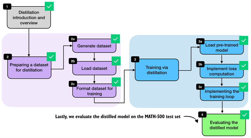 Figure 8.18 The evaluation of the distilled model completes the technical content of this chapter.
This workflow shown in figure 8.18 completes the core technical recipe for distilling a smaller reasoning model from a stronger teacher. In practice, each stage offers room for variation, such as changing how the teacher data is generated and modifying the training settings.
Exercise 8.2: Distilling without
<think>tokens Repeat the distillation experiment without--use_think_tokensand compare the results against the version trained with reasoning traces wrapped in<think>...</think>. Inspect the validation loss and, if possible, evaluate the saved checkpoint on MATH-500. Then compare the results with those listed in table 8.1. How much do the explicit reasoning tags matter in this setup?
8.9 Future directions for reasoning models
Before closing the chapter, let’s discuss where reasoning models are headed next.
For the foreseeable future, the overall broad pattern remains the same. For instance, the general strategy is to develop a stronger reasoning teacher, collect high-quality reasoning traces, and distill them into smaller student models.
One obvious direction is continued refinement of the training recipe popularized by the DeepSeek-R1 paper, which includes both RLVR (chapters 6 and 7) for the flagship models and distillation for the smaller models geared towards computational efficiency.
A second direction is the optimization at inference time. In practice, a reasoning model should not always produce equally long answers. Some tasks benefit from short, direct responses, whereas others benefit from more detailed multi-step reasoning. This creates room for more automatic and flexible inference scaling at the application layer, where the surrounding system decides when to ask for a short answer, when to allocate more reasoning budget, and when to stop early. For example, OpenAI implemented such a system with the launch of GPT-5 in 2025, where they added an “auto” mode to reset the reasoning effort and reasoning trace generation length.
A third direction for improvement is the reward generation for RLVR. Much of the current work still relies heavily on rewards based on final answers, especially in math and code. But process rewards that check intermediate reasoning steps, not just the final result, may provide a richer training signal and help models learn more reliable reasoning strategies. For example, the DeepSeek-Math-V2 paper recently demonstrated that judging the whole answer during training can meaningfully improve reasoning performance.
A fourth direction is the growing role of reasoning models as the engine inside larger agent applications such as OpenAI Codex, Claude Code, and OpenDevin. In these settings, the model must not only solve a simple math or coding problem, but also plan, call tools, recover from failures, and coordinate longer workflows. This naturally pushes reward design beyond math and code correctness. We may want rewards for successful tool use, information retrieval, policy compliance, and more. In turn, this leads to multi-reward training, where several objectives are optimized together instead of relying on a single correctness score.
Distillation will likely remain important in this setting because it offers a practical way to transfer these richer behaviors from larger and more expensive teacher systems into smaller models that are easier to deploy or even run locally while being more cost-effective for users.
8.10 Conclusions
This completes the main technical material of the book. The remaining sections are brief pointers on what to try next, how to keep up with a fast-moving field, and where to find additional material.
8.10.1 What’s next
A practical next step is to start combining the methods from this book instead of treating them as isolated techniques. For example, you could distill a smaller model from a strong teacher, continue training it with RLVR, and then apply inference-time scaling methods such as self-consistency or self-refinement at deployment time. Running these kinds of comparisons is often the fastest way to develop intuition for which method helps most in a given setting.
The appendices are also a good place to continue. They cover additional topics such as LLM architecture details, batched execution for higher throughput, and alternative evaluation approaches.
Lastly, the supplementary code repository (https://github.com/rasbt/reasoning-from-scratch) includes bonus material and standalone scripts that are better suited for longer runs and larger experiments than a notebook.
8.10.2 Staying up to date in a fast-moving field
I hope this book gave you a clearer picture of how modern reasoning models work in practice!
Reasoning-model research is moving quickly, and specific algorithms, datasets, and best practices will continue to change. The core ideas in this book tend to remain relevant and useful. This includes careful model evaluation, distinguishing between inference-time and training-time methods, and a solid understanding of how the training losses and reward signals are computed.
When new methods appear, it helps to map them back to these fundamentals. Many new techniques are best understood as variations or combinations of the building blocks we implemented here, even when the surrounding training recipe becomes more complex.
If you want to stay up to date with the most recent developments in the field, I also regularly write about AI and LLM topics on my blog at https://magazine.sebastianraschka.com.
8.11 Summary
- Distillation trains a smaller student LLM on outputs produced by a larger teacher LLM.
- Hard distillation is usually more practical than soft distillation because teacher logits are often unavailable and teacher text outputs are much cheaper to store and reuse.
- We used DeepSeek-R1 as the teacher model and Qwen3 0.6B as the student model.
- The distillation dataset was built from the 12,000 MATH training problems that do not overlap with MATH-500.
- Each training sample combines a rendered prompt with the teacher reasoning trace and final answer, optionally separated via
<think>...</think>tags. - For efficiency, we tokenize the dataset once, filter it by sequence length, and reuse the processed examples across multiple epochs.
- The training objective is answer-only cross-entropy, which is equivalent to the negative average log-probability of the correct next tokens.
- The distillation training loop is a standard supervised learning loop, which includes shuffling the training examples each epoch, computing the loss, backpropagating, updating the model weights, and tracking validation loss.
- The validation loss is the main signal to watch during training, and saved checkpoints can later be evaluated on MATH-500 with the verifier from chapter 3.
- The distillation approach in this chapter improves the Qwen3 0.6B base model from 15.2% accuracy on MATH-500 to 45.0% accuracy.