Improving reasoning with inference-time scaling
- This chapter covers
- 4.4.1 Understanding the process of selecting the next token
- 4.4.2 Rescaling token scores (logits) via a temperature parameter
- 4.4.3 Sampling the next token from a probability distribution
- 4.4.4 Adding temperature scaling to the text generation function
- 4.5.1 Selecting a subset of top-p tokens
- 4.5.2 Adding a top-p filter to the text generation function
Chapter 4: Improving reasoning with inference-time scaling
This chapter covers
- Prompting an LLM to explain its reasoning to improve answer accuracy
- Modifying the text generation function to produce diverse responses
- Improving reasoning reliability by sampling multiple responses
Reasoning performance and answer accuracy can be improved without retraining or modifying the model itself. These methods operate during inference, when the model generates text. As shown in the overview in figure 4.1, in this chapter, we cover two inference-time scaling methods. As we will see later in this chapter, both methods more than double the accuracy of the base model we used in previous chapters.
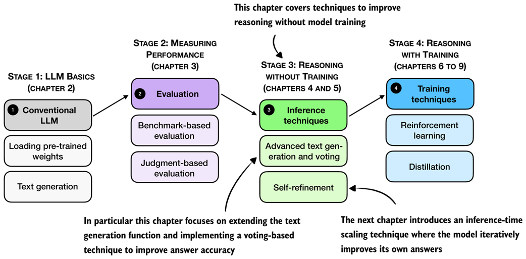 Figure 4.1 A mental model of the topics covered in this book. This chapter focuses on techniques that improve reasoning without additional training (stage 3). In particular, it extends the text-generation function and implements a voting-based method to improve answer accuracy. The next chapter then introduces an inference-time scaling approach where the model iteratively refines its own answers.
The next section provides a general introduction to inference-time scaling before discussing the inference methods that are shown in figure 4.1 in more detail.
4.1 Introduction to inference-time scaling
In general, there are two main strategies to improve reasoning:
- Increasing training compute and
- increasing inference compute (also known as inference-time scaling or test-time scaling).
(In machine learning and AI, “compute” refers to the computational resources required to train or run a model.) These two approaches are illustrated in figure 4.2.
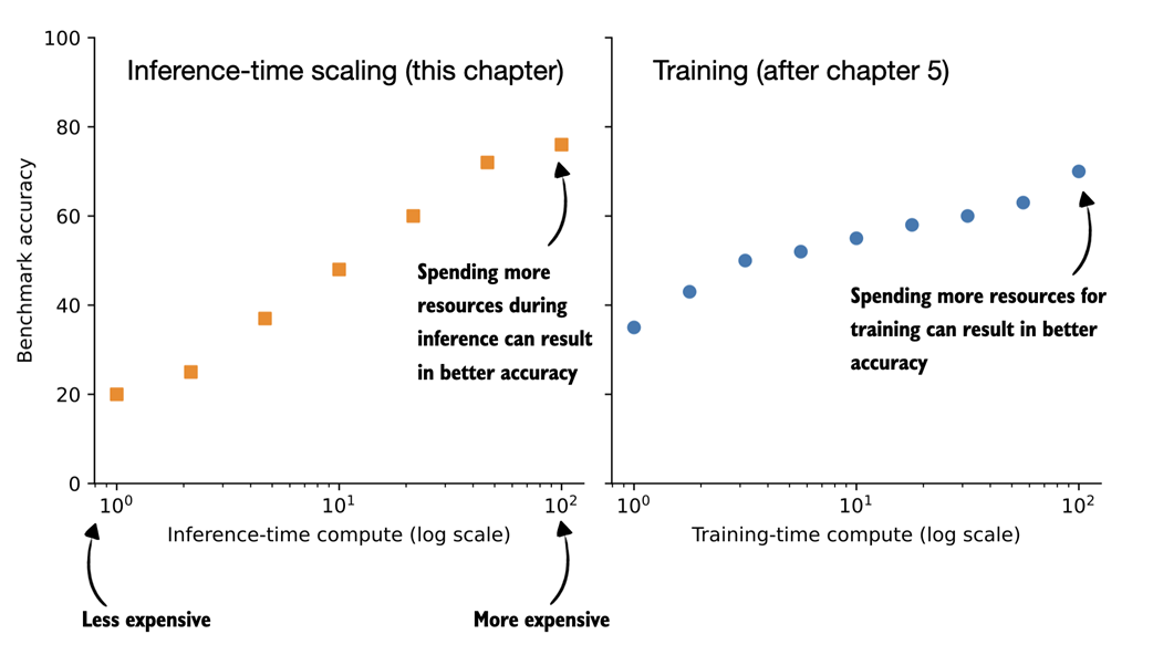 Figure 4.2 Comparison of inference-time scaling (this chapter) and training-time scaling (after chapter 5). Both improve accuracy by using more compute, but inference-time scaling does this on the fly, without changing the model’s weight parameters. The plots are inspired by OpenAI’s article introducing their first reasoning model (https://openai.com/index/learning-to-reason-with-llms/).
The plots shown in figure 4.2 make it seem easy to improve reasoning either by increasing training-time compute or inference-time compute. However, LLMs are usually designed to improve reasoning by combining heavy training-time compute (a topic of future chapters) and increased inference-time compute (the topic of this chapter).
Inference-time compute scaling (also called inference-time scaling and test-time compute scaling) is a broad category that describes any technique that expends more resources to get better answers from the model. This includes making the model generate more tokens and “think” longer, sample multiple answers, or successively refine its answer.
In this book, we focus on three practical and foundational inference-time techniques (figure 4.3):
- Method 1: Extending the chain-of-thought response to prompt the model to explain its reasoning. This is a simple technique that can substantially improve accuracy.
- Method 2: Parallel sampling via self-consistency, where the model generates multiple responses and selects the most frequent one.
- Method 3: Iterative self-refinement, where the model reviews and improves its own reasoning and answers across multiple steps. (This topic is implemented and covered in more detail in the next chapter.)
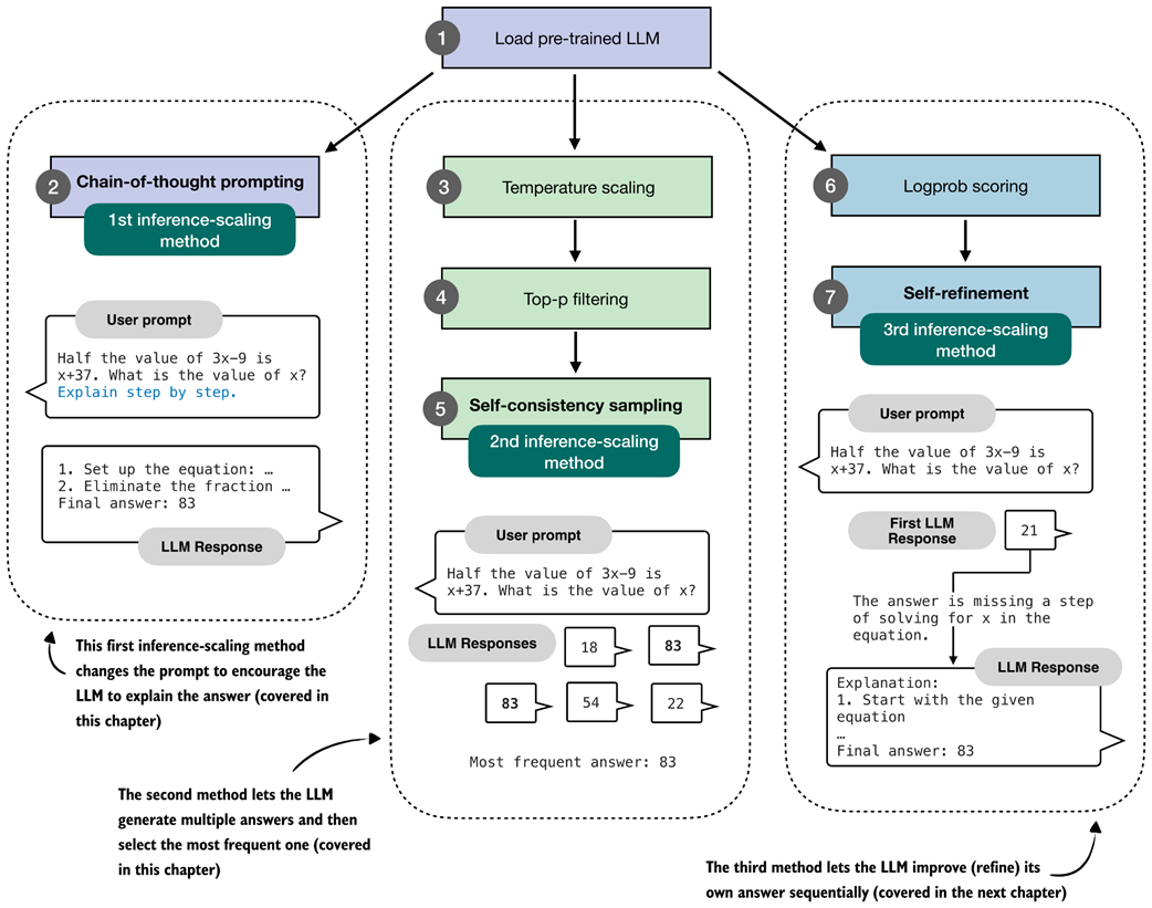 Figure 4.3 Overview of three inference-time methods to improve reasoning covered in this book. The first modifies the prompt to encourage step-by-step reasoning, and the second samples multiple answers and selects the most frequent one. Both are discussed in this chapter. The third method, in which the model iteratively refines its own response, is introduced in the next chapter.
The methods shown in figure 4.3 fall under the category of inference-time scaling because they cause the model to generate more tokens, which increases compute resources during inference. In other words, these methods achieve better accuracy while making the inference process more expensive, which is a common theme of inference-time scaling techniques.
The first method in this chapter improves answer accuracy by prompting the model to explain its reasoning, a simple yet highly effective approach.
Next, we extend the text generation function introduced earlier to enable sampling multiple responses for the same input (the 2nd method shown in figure 4.3). Using this modified function, we implement self-consistency, a voting-based inference-time scaling technique that increases answer accuracy by generating multiple answers and selecting the most frequent one.
In total, I evaluated more than ten different inference-time scaling techniques across thousands of experiments. The three methods illustrated in figure 4.3 were chosen because they offer strong improvements, but also because they are popular and representative of the main paradigms: generating longer responses and generating multiple responses.
Longer responses that include reasoning and explanations (methods 1 and 3) are what we typically expect from reasoning models, as discussed in previous chapters. And parallel sampling (method 2) is also widely used in production systems, such as Claude 4 (as described in https://www.anthropic.com/news/claude-4).
4.2 Loading a pre-trained model
Before we begin implementing the inference-time scaling methods described in the previous section, we load the pre-trained base model we used in the previous sections.
Listing 4.1 Load tokenizer and base model
import torch
from reasoning_from_scratch.ch02 import get_device
from reasoning_from_scratch.ch03 import (
     load_model_and_tokenizer
)

device = get_device()
device = torch.device("cpu")

model, tokenizer = load_model_and_tokenizer(
    which_model="base",
    device=device,
    use_compile=False
)
The code in listing 4.1 loads the model and tokenizer we are using in this chapter. It is similar to the code we used in previous chapters.
Since the code in this chapter is cheap to run, I recommend running this chapter on the "cpu" device for the first time to get the same results as shown in this chapter (running this chapter on a GPU can subtly alter the results.)
Let’s try the model on a prompt from the MATH-500 dataset, which we worked with in the previous chapter:
from reasoning_from_scratch.ch03 import render_prompt

raw_prompt = (
    "Half the value of $3x-9$ is $x+37$. "
    "What is the value of $x$?"
)
prompt = render_prompt(raw_prompt)
print(prompt)
The formatted prompt is as follows:
You are a helpful math assistant.
Answer the question and write the final result on a new line as:
\boxed{ANSWER}

Question:
Half the value of $3x-9$ is $x+37$. What is the value of $x$?

Answer:
We can use the prompt above as input to the generate_text_stream_concat we defined in the previous chapter. However, we will add a subtle modification to this text generation function that will allow us to plug in the advanced text generation function later. The changes are highlighted via the code comments in listing 4.2:
Listing 4.2 Modified generate_text_stream_concat function
from reasoning_from_scratch.ch02 import generate_text_basic_stream_cache


def generate_text_stream_concat_flex(
    model, tokenizer, prompt, device, max_new_tokens,
    verbose=False,
    generate_func=None,
    **generate_kwargs
):

    if generate_func is None:
        generate_func = generate_text_basic_stream_cache

    input_ids = torch.tensor(
        tokenizer.encode(prompt), device=device
        ).unsqueeze(0)

    generated_ids = []
    for token in generate_func(
        model=model,
        token_ids=input_ids,
        max_new_tokens=max_new_tokens,
        eos_token_id=tokenizer.eos_token_id,
        **generate_kwargs,
    ):
        next_token_id = token.squeeze(0)
        generated_ids.append(next_token_id.item())

        if verbose:
            print(
                tokenizer.decode(next_token_id.tolist()),
                end="",
                flush=True
            )
    return tokenizer.decode(generated_ids)
In short, the generate_text_stream_concat_flex function above is similar to the generate_text_stream_concat function from the previous chapter, except that we can now pass in the text generation function (like generate_text_basic_stream_cache) as a function argument instead of hard-coding it. In future sections, we will swap the generate_text_basic_stream_cache function with more advanced functions.
The usage is also similar to before, except that we can now pass the text generator function (for example, generate_text_basic_stream_cache) explicitly:
response = generate_text_stream_concat_flex(
    model, tokenizer, prompt, device,
    max_new_tokens=2048, verbose=True,
    generate_func=generate_text_basic_stream_cache
)
The generated output is:
\boxed{20}
Note that the answer is wrong, and the correct solution is 83. In the remainder of this chapter, and the next chapter, we will implement inference-time scaling methods to get the model to generate the correct answer.
4.3 Generating better responses with chain-of-thought prompting
After loading the pre-trained base model in the previous section and setting up the text generation function, this section focuses on improving the model output via so-called chain-of-thought prompting.
Chain-of-thought prompting is a classical yet simple and effective technique that modifies the input prompt to encourage the LLM to generate an explanation or so-called chain-of-thought (also called reasoning chain), as illustrated in figure 4.4.
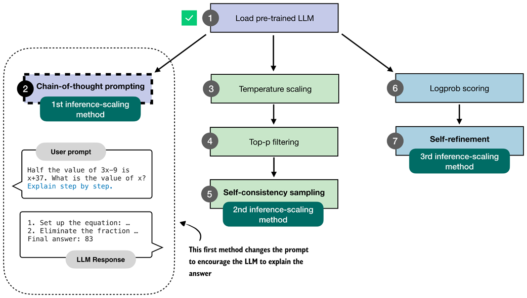 Figure 4.4 The first inference-time method, chain-of-thought prompting, modifies the prompt to encourage the model to explain its reasoning step by step before producing a final answer.
The simplest way to try chain-of-thought prompting is to append a phrase like "Explain step by step." to the prompt, as shown below:
prompt_cot = prompt + " \n\nExplain step by step."

response_cot = generate_text_stream_concat_flex(
    model, tokenizer, prompt_cot, device,
    max_new_tokens=2048, verbose=True,
)
The response is now as follows:
To solve the problem, we need to find the value of \( x \) such that
half the value of \( 3x - 9 \) is equal to \( x + 37 \).

# ...

### Step 3: Solve for \( x \)
Subtract \( 2x \) from both sides to isolate \( x \):
\[
3x - 2x - 9 = 74
\]
Simplify:
\[
x - 9 = 74
\]
Add 9 to both sides to solve for \( x \):
\[
x = 74 + 9
\]
\[
x = 83
\]

### Final Answer:
\[
\boxed{83}
\]
As we can see, the model now writes a lengthy step-by-step explanation and, in this case, now arrives at the correct answer.
This simple chain-of-thought prompting is a good demonstration of the inference-time scaling trade-off. While the model now answers correctly, it expends many more tokens than before, which makes the model much more compute-intensive or costly in practice.
Note that while the model generates the correct answer in this case, not all problems benefit from chain-of-thought prompting. On simple problems, it can even sometimes degrade the model’s performance, as the model might sometimes generate erroneous explanations and mislead itself. This phenomenon is also known as “overthinking.”
Lastly, not every model benefits from the “Explain step by step” (or similar) instruction. In this case, we use a simple base model that doesn’t always generate explanations, so chain-of-thought prompting can clearly help. However, trained reasoning models, such as the “reasoning” variant of the Qwen3 model we used in the exercises of the previous chapter, already write explanations alongside their responses and don’t need or benefit from this type of chain-of-thought prompting.
Why chain-of-thought can improve accuracy
Chain-of-thought prompting asks the model to write out the intermediate steps that lead to a final answer. This helps in two practical ways.
First, walking through the steps gives the model more opportunities to correct itself.
Second, step-by-step reasoning matches how many training examples are written. For instance, large math and logic datasets often contain detailed solutions, so asking for a chain of thought aligns the model with patterns it has already learned.
At the same time, chains-of-thought are not a guarantee for correctness. It can produce wrong reasoning, and for very simple problems it may even introduce unnecessary steps that lead to more mistakes. In other words, chains-of-thought can improve accuracy on many reasoning tasks, but it is not universally beneficial.
Overall, chain-of-thought answering does not provide the model with new knowledge, but it changes how the model uses its existing knowledge. Often, this shift can lead to more reliable answers. This is especially true for math, code, logic problems, and other sorts of multi-step problems.
Exercise 4.1: Use chain-of-thought prompting on MATH-500
Modify the
evaluate_math500_streamfunction in section 3.9 of chapter 3 to see if chain-of-thought prompting improves the MATH-500 accuracy of the base model.
4.4 Controlling output diversity with temperature scaling
The previous section gave a brief taste of inference-time scaling by extending the model’s answer via chain-of-thought prompting. Chain-of-thought prompting can be seen as a sequential technique as we extend the number of next-token prediction steps.
In the remainder of this chapter, we will implement a technique that generates multiple answers, as illustrated in figure 4.5. Since the answers are independent of each other, this can be implemented as a parallel sampling (if we have the necessary resources, for example, using multiple GPUs), which in this case wouldn’t increase the wait time for a user to get the answer.
(Note that chain-of-thought prompting can also be combined with this technique, but more on that in a later section.)
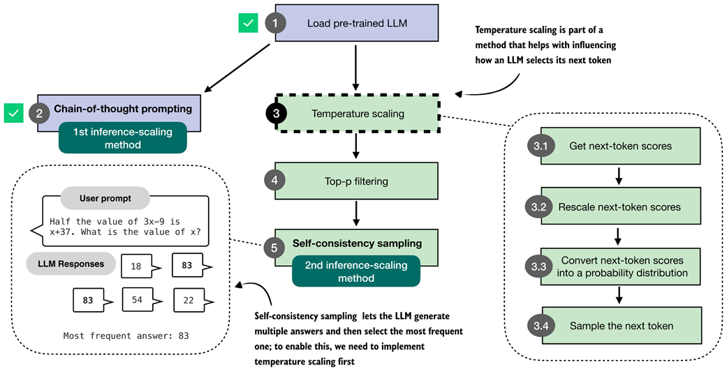 Figure 4.5 The second inference-time method, self-consistency sampling, generates multiple answers and selects the most frequent one. This method relies on temperature scaling, covered in this section, which influences how the model samples its next token.
The self-consistency technique, illustrated in figure 4.5 and covered in this chapter, is also called self-consistency sampling and was formally described in the Google Research paper Self-Consistency Improves Chain-of-Thought Reasoning in Language Models (https://arxiv.org/abs/2203.11171).
Before implementing self-consistency sampling (step 5 in figure 4.5), we first need to extend the text generation function so that it can produce multiple different answers for the same prompt. To achieve this, we will implement two techniques, temperature scaling (step 3) and top-p filtering (step 4), which allow the model to sample different responses.
Temperature scaling is the main focus of this section. Before we get to temperature scaling, the next subsection provides a brief overview of how the next token is sampled in an LLM.
4.4.1 Understanding the process of selecting the next token
This subsection gives a closer look at the text generation process we implemented so far and explains how the next-token selection process works under the hood. This information will help you understand the motivation behind temperature scaling.
For instance, suppose we have the following simple prompt:
ex_prompt = "The capital of Germany is"

response = generate_text_stream_concat_flex(
    model, tokenizer, ex_prompt, device,
    max_new_tokens=1, verbose=True
)
The model’s response is " Berlin".
While this looks relatively simple, there are multiple steps happening under the hood, as illustrated in figure 4.6.
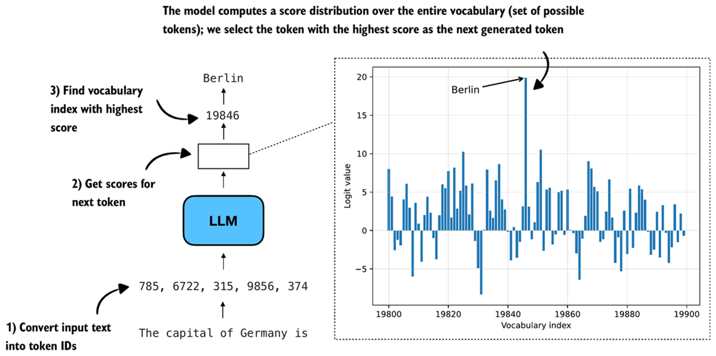 Figure 4.6 Illustration of how an LLM generates the next token. The model converts the input into token IDs, computes scores for all possible next tokens, and selects the one with the highest score as the next output.
When generating text, as discussed in chapter 2, the inputs are first converted into token IDs:
input_token_ids = torch.tensor(
    tokenizer.encode(ex_prompt), device=device
).unsqueeze(0)
print(input_token_ids)
In this case, the token IDs are
tensor([[ 785, 6722, 315, 9856, 374]])
In the second step (step 2 in figure 4.6), we get the scores for the output token we want to generate. These model output scores are also called logits. Note that an LLM generates one output token for each input token, but we are only interested in the last token, which we select via the [:, -1] tensor indexing. This last token corresponds to the token we want to generate:
with torch.inference_mode():
    next_token_logits = model(input_token_ids)[:, -1]
print(next_token_logits.shape)
The printed output shape is [1, 151936], where 151936 is the vocabulary size of this tokenizer and model. The vocabulary size contains all the unique tokens the tokenizer can handle and the LLM can generate.
To actually obtain the next generated token (here: " Berlin"), we have to find a vocabulary entry that is associated with the largest score (step 3 in figure 4.6):
max_token_id = torch.argmax(next_token_logits)
print(f"Token ID: {max_token_id}")
print(f"Decoded token: '{tokenizer.decode([max_token_id])}'")
The output is:
Token ID: 19846
Decoded token: ' Berlin'
Above, we covered the three main steps in generating the next token. Before we go to the next section, let us take a closer look at the score distribution of the next_token_logits tensor we passed into torch.argmax function to obtain the token IDs, and plot them in matplotlib:
Listing 4.3 Plotting the next-token logit scores
import matplotlib.pyplot as plt

def plot_scores_bar(
    next_token_logits, start=19_800, end=19_900,
    arrow=True, ylabel="Logit value"
):
    x = torch.arange(start, end)
    logits_section = next_token_logits[0, start:end].float().cpu()

    plt.bar(x, logits_section)
    plt.xlabel("Vocabulary index")
    plt.ylabel(ylabel)

    if arrow:
        max_idx = torch.argmax(logits_section)
        plt.annotate(
            "Berlin",
            xy=(x[max_idx], logits_section[max_idx]),
            xytext=(x[max_idx] - 25, logits_section[max_idx] - 2),
            arrowprops={
                "facecolor": "black", "arrowstyle": "->", "lw": 1.5
            },
            fontsize=10,
        )

    plt.grid(alpha=0.3)
    plt.tight_layout()
    plt.show()

plot_scores_bar(next_token_logits)
Note that we restrict the plot to the 100 vocabulary index tokens between 19,800 and 19,900, rather than plotting the scores for all 151,936 entries, which would make the plot too crowded. (I selected this specific range such that it contains the entry with the highest score.) The resulting plot is shown in figure 4.7.
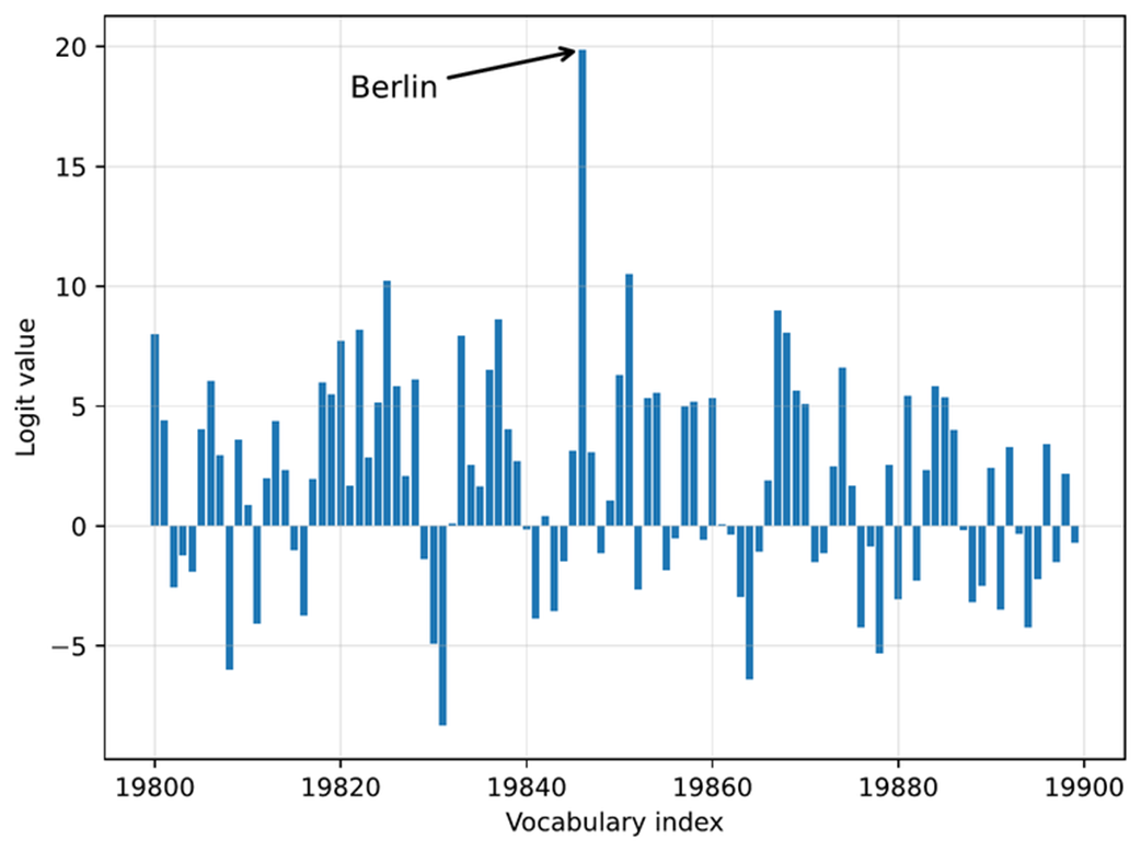 Figure 4.7 Example of next-token logits for a language model. Each bar represents a possible token’s score, with “Berlin” having the highest logit value and being selected as the next token.
The plot in figure 4.7 shows all 100 logit values (scores) for vocabulary indices 19,800-19,899. The values range approximately from -8 to 20, where 20 corresponds to the vocabulary index for the token " Berlin".
4.4.2 Rescaling token scores (logits) via a temperature parameter
Now that we have walked through how the model selects its next token, we can introduce the concept of temperature. Temperature, or rather a chosen temperature parameter, changes how sharp or spread out the logits (token scores) are, which in turn affects how the next token is selected.
As shown in figure 4.8, this section focuses on rescaling the next-token logits with a temperature parameter before using them for sampling. Rescaling here means adjusting the magnitude of the scores so the sampling step becomes more or less sensitive to the score differences.
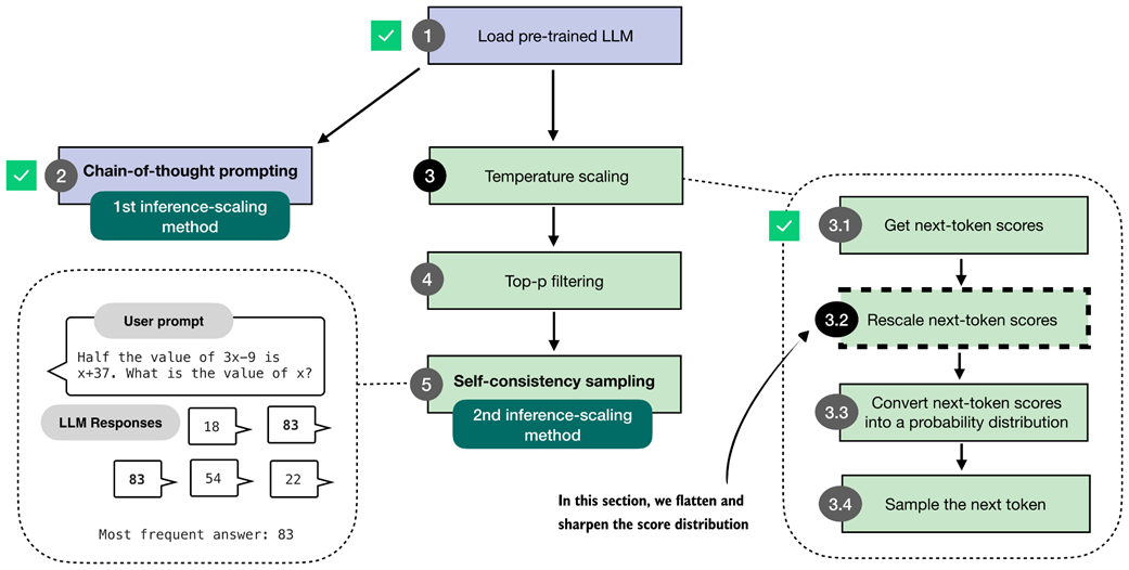 Figure 4.8 In this section, we implement the core part of temperature scaling (step 3.2), which adjusts the next-token scores. This allows us to control how confidently the model selects its next token in later steps.
The code for implementing the temperature rescaling step, step 3.2 in figure 4.8, is relatively short and simple, as shown in listing 4.4 below.
Listing 4.4 Rescaling next-token scores via temperature scaling
def scale_logits_by_temperature(logits, temperature):
    if temperature <= 0:
        raise ValueError("Temperature must be positive")
    return logits / temperature
In essence, the code in listing 4.4 rescales the logit values before converting them to probabilities in the next section.
In practice, temperature values are expected to be positive numbers. A temperature of 1.0 means no change, since dividing a number by 1 is the number itself.
We will add additional temperature scaling safeguards later when we add temperature scaling to our text generation function.
For all other values, the logits are divided by the temperature. A temperature lower than 1.0 makes the distribution sharper (which will make the model more confident when we select the next token in the upcoming sections). Temperatures higher than 1.0 flatten the logits, which can make the sampling (step 3.4 in figure 4.8) more diverse.
Let’s see this scale_logits_by_temperature function in action and try it out with relatively extreme temperature values 0.5 and 5.0 for a stronger effect:
Listing 4.5 Plotting the temperature-rescaled logits
def plot_logits_with_temperature(
    next_token_logits, start=19_800, end=19_900,
    temps=(0.5, 5.0),
):
    x = torch.arange(start, end)
    logits_orig = next_token_logits[0, start:end].float().cpu()

    logits_scaled = [
        scale_logits_by_temperature(logits_orig, T) for T in temps
    ]

    plt.plot(x, logits_orig, label="Original logits", lw=2)
    plt.plot(
        x, logits_scaled[0],
        label=f"T={temps[0]} (sharper)", ls="--", lw=1
    )
    plt.plot(
        x, logits_scaled[1],
        label=f"T={temps[1]} (flatter)", ls=":", lw=3
    )

    # Highlight max logit
    max_idx = torch.argmax(logits_orig)
    plt.annotate(
        "Berlin",
        xy=(x[max_idx], logits_orig[max_idx]),
        xytext=(x[max_idx] - 25, logits_orig[max_idx] + 2),
        arrowprops={"facecolor": "black", "arrowstyle": "->", "lw": 1.5},
        fontsize=12,
    )

    plt.xlabel("Vocabulary index")
    plt.ylabel("Logit value")
    plt.legend()
    plt.grid(alpha=0.3)
    plt.tight_layout()
    plt.show()

plot_logits_with_temperature(
    next_token_logits,
    temps=(0.5, 5.0)
)
As shown in the plot in figure 4.9, the larger temperature (5.0) yields a much flatter score distribution, whereas the smaller temperature (0.5) yields a much sharper one.
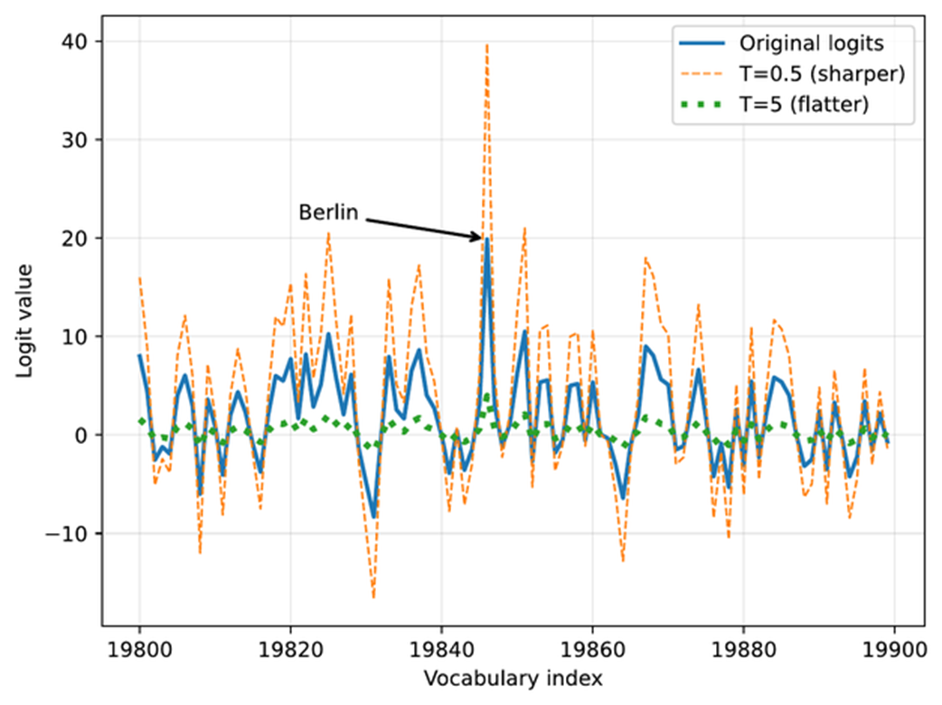 Figure 4.9 The effect of temperature scaling on logits. Lower temperatures make the distribution sharper, while higher temperatures flatten it. (Please note that this visualization is shown as a line plot for readability, though a bar plot would more accurately represent the discrete vocabulary scores.)
Note that the plotting code in listing 4.5 above looks very similar to the plotting code we used in the previous section (listing 4.3). However, in addition to applying the temperature scaling, we now use a line plot (plt.plot) instead of a bar plot (plt.bar). While a bar plot is technically a better choice for the discrete vocabulary indices on the x-axis, the line plot makes it easier to visualize and compare the rescaled logits in this case.
Why temperature?
The term temperature comes from physics, where temperature controls how much randomness or movement there is in a system. In LLMs, we use the same idea to control how confidently or creatively the model chooses its next token, as we will see in the next two sections.
4.4.3 Sampling the next token from a probability distribution
The previous section rescaled the logit values using different temperature values. The purpose of this is that it lets us (later) influence how the model selects the next token.
However, before we get to the next-token sampling portion in the next section, this section adds one more intermediate step: converting the rescaled logits into probability scores, as shown in figure 4.10.
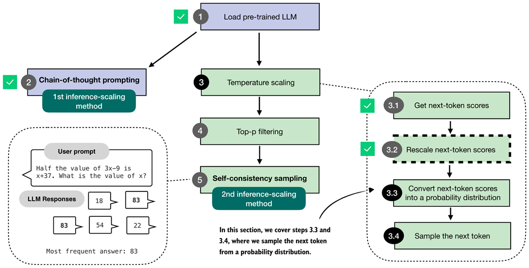 Figure 4.10 Overview of the sampling process for generating tokens. In this section, we focus on steps 3.3 and 3.4, where the next-token scores are converted into a probability distribution, and the next token is sampled based on that distribution.
To demonstrate how rescaled logits are converted into probability scores, as described in step 3.3 of figure 4.10, we will use a temperature of 5.0. This makes it easier to visualize the resulting probabilities in a plot. The " Berlin" token, for example, has such a high logit value that it would otherwise dominate the scale and make it difficult to see the probabilities of the surrounding tokens.
The conversion from rescaled logits to probability scores can be done with a single function call, torch.softmax, as shown in listing 4.6 below.
Listing 4.6 Sampling the next-token from a probability distribution
rescaled_logits = scale_logits_by_temperature(next_token_logits, 5.0)

next_token_probas = torch.softmax(
    rescaled_logits, dim=-1
)
The torch.softmax function in listing 4.6 normalizes the logit values into values in the range between 0 and 1, and such that the values sum to 1, which we can confirm via the following code:
print("Probability sum:", torch.sum(next_token_probas))
Additionally, let’s visualize the converted scores by reusing the plot_scores_bar function from listing 4.3 earlier:
plot_scores_bar(
    next_token_probas, arrow=False, ylabel="Probability value"
)
The resulting plot, now with the probability values on the y-axis, is shown in figure 4.11.
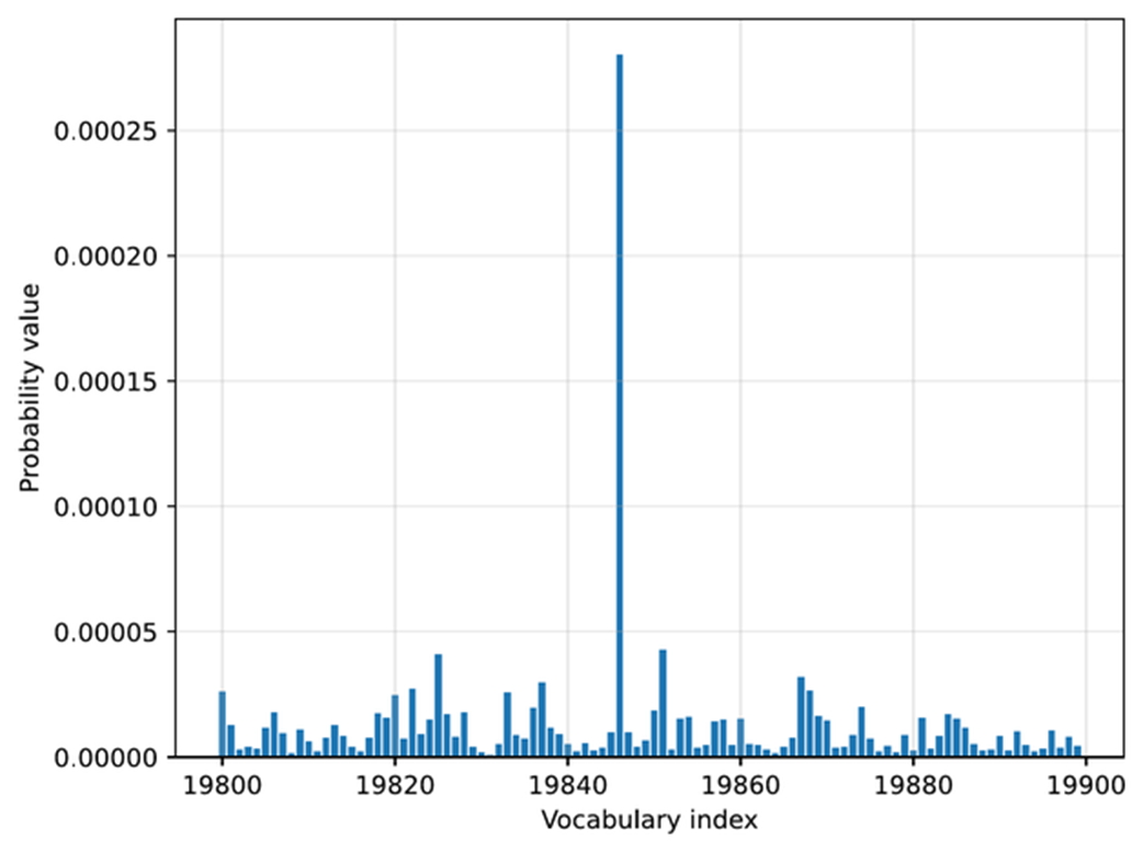 Figure 4.11 Token probabilities obtained by applying the softmax function to the rescaled logits. The token of the highest probability (corresponding to
 " Berlin", but with the label omitted for code simplicity) is selected as the next output.
In the plot in figure 4.11, we can see that the token ID 19,846 (“ Berlin”) has the highest value in this selected vocabulary range. The probability is 0.0003, which we can confirm via the following code:
print("Token ID 19,846 probability:", next_token_probas[:, 19846])
Note that while this 0.0003 value is relatively small, there is no other value larger than this outside the selected vocabulary range in this plot. For instance, using the following code, we can confirm that 0.0003 is indeed the largest value:
print("Highest probability:", max(next_token_probas.squeeze(0)))
We can interpret this score as the model’s confidence. This means that the model is more confident in " Berlin" (19,846) as the next token than in other tokens.
The reason the value is so small is that we are using a large temperature, which makes it easier to compare this value next to the other token values. However, if we change the temperature from 5 to 0.5, the probability score increases from 0.0003 to 0.3398, and the probability scores of the other tokens will be even closer to 0.
The softmax function under the hood
The softmax function converts a vector of raw scores (logits) into a probability distribution where each value lies between 0 and 1, and all values sum to 1. This conversion makes it easier to interpret them and sample from them later.
If you are familiar with mathematical notation, the formula behind the softmax function is
\[\text{softmax}(z_i) = \frac{\exp(z_i)}{\sum_j \exp(z_j)}\]Here, z is a vector of real-valued inputs
\[z = [z_1, z_2, \dots, z_n]\]where
- $n$ is the number of elements in the vector,
- $j$ is the index of the current element ($1 \le j \le n$),
- $i$ is the index used to sum over all elements ($1 \le i \le n$),
This produces a normalized probability for each element $a_i$, such that
\[\sum_i \text{softmax}(z_i) = 1\]In code, the softmax function can be implemented with a simple 3-liner:
def softmax_with_temperature(logits, temperature):
    scaled_logits = logits / temperature
    return torch.softmax(scaled_logits, dim=0)
However, in practice, we prefer the
torch.softmaxfunction because it has some additional numerical stability improvements to handle very small and very large values more reliably.
The purpose of converting the logits into these probability scores is that the probability scores are somewhat more interpretable, and we can now sample from them using a torch.multinomial function.
For instance, if we draw one sample from this probability distribution, we have a 0.03% chance of getting " Berlin" with our temperature setting of 5.0 (and a 33.98% chance of getting " Berlin" with a temperature of 0.5).
The sampling process, corresponding to step 3.4 in the figure at the beginning of this section, can be implemented as follows:
torch.manual_seed(123)
print(
    "Sampled token:",
    torch.multinomial(next_token_probas.cpu(), num_samples=1)
)
This code returns token ID 65,094, which corresponds to the word " mistress". Note that the word doesn’t make sense in our context, "The capital of Germany is", and it was selected randomly in this case and influenced by the high-temperature setting, which encourages tokens other than " Berlin" to be sampled.
The torch.multinomial function samples the vocabulary indices proportional to their probabilities. In other words, vocabulary indices with higher probabilities are more likely to be sampled. If we repeated the sampling a very large number of times, we would sample the vocabulary index corresponding to the token " Berlin" with 0.03% probability, given a temperature of 5.
Before we look at some additional examples, note that we specified a random seed above to make the code in this chapter reproducible. However, the torch.multinomial() function may still yield different results on "cuda" and "mps" devices, and may even crash when we draw larger numbers of samples (I observed this issue in PyTorch 2.9 on both "cuda" and "mps" devices), which is why we run the sampling on the CPU via .cpu().
Let’s now sample more next-token candidates to get a more representative sample.
Listing 4.7 Sampling multiple next-token candidates
def count_samples(probas, num_samples=1000, threshold=1, tokenizer=None):
    samples = torch.multinomial(
        probas.cpu(), num_samples=num_samples, replacement=True
    )
    counts = torch.bincount(samples.squeeze(0), minlength=1)

    for i, c in enumerate(counts):
        if c > threshold:
            if tokenizer is None:
                print(f"Vocab index {i}: {c.item()}x")
            else:
                print(f"'{tokenizer.decode([i])}': {c.item()}x")
This count_samples function in listing 4.7 samples token indices from a probability distribution and counts how often each token is drawn. It uses torch.multinomial to randomly select num_samples indices proportional to their probabilities. The replacement=True setting allows us to draw the same token multiple times.
Then, torch.bincount counts how often each index appears. Finally, it prints only tokens that occur more than a specified threshold, so that it doesn’t clutter the output with more infrequently drawn tokens.
Multinomial sampling
Multinomial sampling is the procedure used to pick the next token given a probability distribution over the vocabulary, like the softmax probability scores. In multinomial sampling, instead of always selecting the most likely token (known as greedy decoding), we draw one token at random, where tokens with higher probability are more likely to be selected. This randomness is important for generating diverse responses, which we later use in self-consistency.
To illustrate it further we can think of the probability scores as a set of weighted choices. For example, a token with probability 0.40 is four times as likely to appear as one with probability 0.10, but both remain possible outcomes.
Suppose the model assigns the following probabilities:
- “Berlin”: 0.70
- “Munich”: 0.20
- “Hamburg”: 0.10
Greedy decoding would always return “Berlin.”
Multinomial sampling instead draws one token according to these weights. Across a very large number of draws, “Berlin” will appear most often (70% of the time), “Munich” sometimes (20% of the time), and “Hamburg” only occasionally (10% of the time).
This variability is what allows us to generate multiple candidate answers for self-consistency in later sections.
Please note that the count_samples function is meant for illustration only. It draws many samples from the distribution so you can see how often each token is selected. In real text generation we only draw one token at a time, but taking a large number of samples here makes the underlying probabilities easier to visualize and understand.
First, let’s run the count_samples function on the probability scores that we obtained by applying a temperature of 5:
torch.manual_seed(123)
count_samples(next_token_probas, tokenizer=tokenizer)
The output is as follows:
'}': 2x
' </': 2x
' represent': 2x
' Inf': 2x
'()*': 2x
' beside': 2x
' Kob': 2x
'': 2x
As we can see, even though the default sample size is 1000, none of the sampled tokens appear more than 2 times. Also, these are all nonsense tokens in the context of the "The capital of Germany is" query. The reason for these nonsensical results is that we used a temperature value that is much too high.
Let’s try a lower temperature value of 0.35, which makes the score distribution sharper, and which makes it more likely to select a meaningful next token:
torch.manual_seed(123)
probas_lowT = torch.softmax(
    scale_logits_by_temperature(next_token_logits, 0.35), dim=-1
)
In this case, we see the following output:
' __': 158x
' Berlin': 435x
' ____': 169x
' ______': 209x
' Munich': 3x
' Hamburg': 3x
' _____': 18x
The output makes a lot more sense as next-token candidates for our "The capital of Germany is" query. Out of the 1000 samples, the token " Berlin" was drawn 435 times. You can check via print(probas_lowT[0, 19_846]) that the probability of drawing this token is approximately 42% given the temperature value 0.35. To make it even more likely that " Berlin" is sampled, we could further reduce the temperature.
Notice that some of the other rare candidates also make sense, for example, both " Munich" and " Hamburg" are big cities in Germany, so they are not completely unrelated to the query. The underscored responses (" ____") are likely due to the model having seen text in the form of a quiz with a placeholder, e.g., "The capital of Germany is ____".
You may wonder, if " Berlin" is the correct answer, what’s the point in making the model occasionally give the wrong answer by adding this temperature-rescaling and multinomial sampling?
In general, for different kinds of queries, introducing randomness during sampling helps the model explore alternative responses instead of always choosing the single most likely token. This variability can be useful for creative or open-ended tasks, where there may be multiple valid completions.
Specifically, in reasoning tasks, we can leverage this sampling diversity through techniques such as self-consistency (section 4.6), which generate multiple candidate answers and compare them to improve answer accuracy.
4.4.4 Adding temperature scaling to the text generation function
Before we move to the next section and introduce another improvement to the text generation process by adding a token-probability selection filter, let’s add the temperature scaling modification to the text generation function so we can use it more readily when generating new tokens via the model.
Listing 4.8 Text generation with temperature scaling
from reasoning_from_scratch.qwen3 import KVCache

@torch.inference_mode()
def generate_text_temp_stream_cache(
    model,
    token_ids,
    max_new_tokens,
    eos_token_id=None,
    temperature=0.
):
    model.eval()
    cache = KVCache(n_layers=model.cfg["n_layers"])
    model.reset_kv_cache()

    out = model(token_ids, cache=cache)[:, -1]
    for _ in range(max_new_tokens):

        ########################################
        # NEW:
        orig_device = token_ids.device

        if temperature is None or temperature == 0.0:
            next_token = torch.argmax(out, dim=-1, keepdim=True)

        else:
            logits = scale_logits_by_temperature(out, temperature)
            probas = torch.softmax(logits, dim=-1)
            next_token = torch.multinomial(probas.cpu(), num_samples=1)
            next_token = next_token.to(orig_device)

        #########################################
        if (eos_token_id is not None
                and torch.all(next_token == eos_token_id)):
            break

        yield next_token
        out = model(next_token, cache=cache)[:, -1]
The generate_text_temp_stream_cache in listing 4.8 is similar to the generate_text_stream_cache function from the chapter 2 exercises, which we also used in chapter 3. What’s new is that we have now inserted the temperature rescaling and sampling. The new parts are below the # New comment indicator in the code.
torch.manual_seed(123)
response = generate_text_stream_concat_flex(
    model, tokenizer, prompt, device,
    max_new_tokens=2048, verbose=True,
    generate_func=generate_text_temp_stream_cache,
    temperature=1.1
)
The output is \boxed{$x = \frac{90}{7}$}. The correct answer is 83, so the model is still wrong, but this was more meant as a demonstration that we can tweak the answer by using temperature scaling and sampling.
In the next section, we will learn how to improve the sampling process.
4.5 Balancing diversity and coherence with top-p sampling
In the previous section, we saw how temperature scaling and sampling (via torch.multinomial) can increase the diversity of the LLM responses, for better or for worse. Specifically, we saw that using the approach described in the previous section, we may end up sampling “weird” tokens that are unrelated to the user query.
In this section, we improve the sampling process by adding a top-p filter (figure 4.12) such that very low-confidence tokens are not sampled by accident. The top-p sampling process described in this section is also known as nucleus sampling.
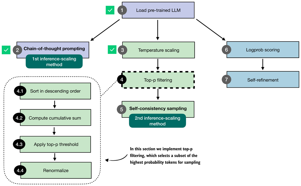 Figure 4.12 Overview of the top-p filtering process. The filter keeps only the highest-probability tokens by sorting them, applying a cumulative cutoff, selecting the top-p subset, and renormalizing the result.
Figure 4.12 summarizes the four steps that make up the top-p filter: sorting the token probabilities (4.1), computing their cumulative sum (4.2), selecting the subset that satisfies the top-p cutoff (4.3), and renormalizing the remaining probabilities so that they again form a valid distribution (4.4).
The renormalization step is necessary because, once we remove all low-probability tokens, the remaining probabilities no longer sum to one. To sample correctly, we rescale these remaining values so that they represent a proper probability distribution.
Having outlined the full top-p filtering pipeline in figure 4.12, the next subsections walk through each step in detail. We will start with a brief recap of temperature scaling and then implement steps 4.1 to 4.4 that are shown in figure 4.12.
4.5.1 Selecting a subset of top-p tokens
In this section, we implement the top-p filter illustrated in figure 4.12 that we will use to improve the text generation function, which we plan to use for self-consistency sampling.
Note
The purpose of top-p filtering in this section is to drop low-probability tokens so that only the most plausible options remain during sampling. This reduces the chance of producing tokens that do not fit the context.
Before we implement the top-p filter, let us briefly recap the temperature-scaling and sampling process with a simpler toy dataset, which makes it easier to illustrate the process. For instance, let’s assume the models’ and tokenizer’s vocabularies have only 10 entries, rather than 151,936.
Listing 4.9 Recap of temperature scaling and sampling with toy data
toy_logits = torch.tensor(
    [-0.7, -3.0, 0.1, -1.2, 2.0, -1.0, -0.5, -2.0, 0.3, 1.5]
)

toy_logits_scaled = scale_logits_by_temperature(toy_logits, 1.0)
toy_probas = torch.softmax(toy_logits_scaled, dim=-1)

plt.bar(
    torch.arange(len(toy_probas)), toy_probas,
    alpha=0.5
)

plt.ylim([0, 1])
plt.xlabel("Vocabulary index")
plt.ylabel("Probability")
plt.show()
Please note that the toy_logits variable holds the example values that we would get for the next-token logit scores via the model(token_ids, cache=cache)[:, -1] call in the previous section, assuming that the vocabulary size is 10. The resulting plot is shown in figure 4.13.
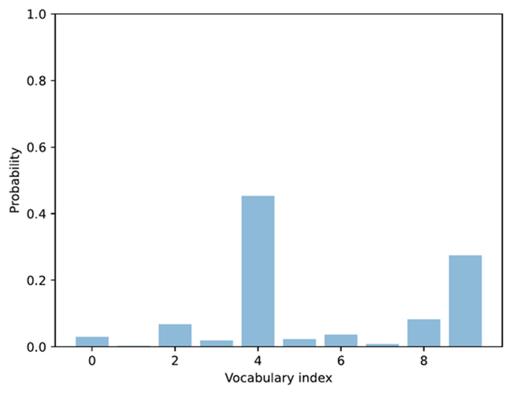 Figure 4.13 Example of token probabilities before top-p filtering. The distribution includes many low-probability tokens, which will later be truncated by applying a cumulative probability threshold.
The bar plot in figure 4.13 shows the next-token logit scores after rescaling them to a probability score. So far, this is a recap of the previous section. Next, we will add the first two top-p filtering steps (steps 4.1 and 4.2) illustrated in figure 4.12. This involves sorting the probability scores in descending order and computing the cumulative sum.
Listing 4.10 Compute cumulative probability sum
sorted_probas, sorted_idx = torch.sort(toy_probas, descending=True)
cumsum = torch.cumsum(sorted_probas, dim=-1)

plt.bar(
    torch.arange(len(sorted_probas)), sorted_probas,
        alpha=0.5
)
plt.step(
    torch.arange(len(cumsum)), cumsum,
    where="mid", color="C1", label="Cumulative sum"
)

plt.ylim([0, 1])
plt.xlabel("Token rank (sorted by probability)")
plt.ylabel("Probability")
plt.show()
The torch.cumsum function used in listing 4.10 above computes the cumulative sum of elements along a given dimension. In this example, it takes the sorted token probabilities and adds them up step by step, so each position in torch.cumsum represents the total probability accumulated up to that token.
For instance, the first element equals the highest probability, the second equals the sum of the top two, and so on, until the final value reaches 1. This is best explained by looking at the cumulative step plot, produced by the code in listing 4.10 and shown in figure 4.14.
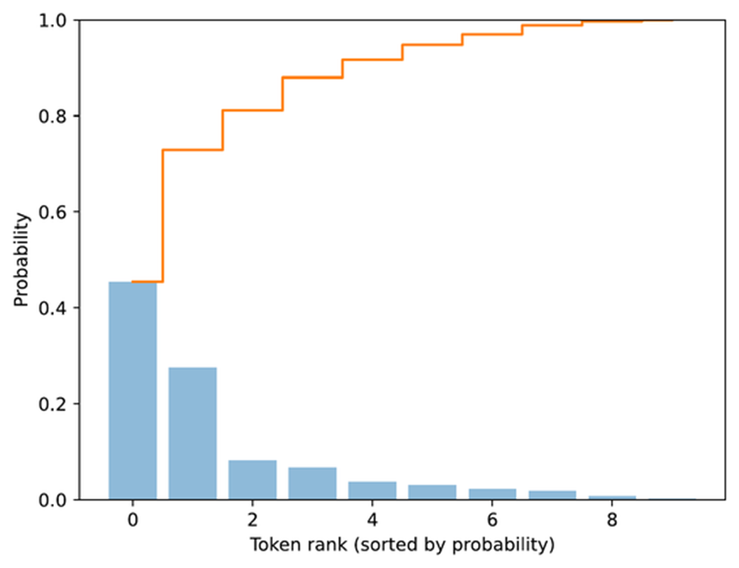 Figure 4.14 Visualization of sorted token probabilities and their cumulative sum. This step prepares for top-p filtering by showing how probabilities accumulate when ordered from highest to lowest, which helps determine where to set the cutoff threshold.
Now that we have the cumulative probability sum, we can implement the core top-p filtering step. The “p” in top-p stands for probability, and top-p can be translated to “keep the smallest set of tokens whose cumulative probability stays below or equal to p.” A simple code implementation of top-p filtering may look as follows:
Listing 4.11 A simple-top-p filtering rule
top_p = 0.8
keep_mask = cumsum <= top_p
n_kept = torch.sum(keep_mask).item()
print("Cumulative sum:", cumsum)
print("Tokens kept:", n_kept)
In code, this is implemented as keep_mask = cumsum <= top_p, which marks all tokens whose cumulative probability mass does not yet exceed the threshold p (here, defined via top_p=0.8). The number of retained tokens is then computed and assigned to the variable n_kept. The output is
Cumulative sum: tensor([0.4538, 0.7290, 0.8119, 0.8798,
0.9170, 0.9475, 0.9701, 0.9886, 0.9969, 1.0000])
Tokens kept: 2
Looking at the returned cumulative probabilities, the second entry (0.7290) is just below the top-p threshold of 0.8, and the third entry (0.8119) exceeds it, which is why only the first 2 tokens are kept.
Now, a more common variant of top-p filtering includes the token that exceeds the threshold:
Listing 4.12 A common top-p filtering variant
keep_mask = (cumsum - sorted_probas) < top_p
n_kept = keep_mask.sum().item()
print("Tokens kept:", n_kept)
This code now returns 3 as the number of tokens kept. This follows the definition of top-p filtering that the smallest set of tokens is kept such that the cumulative probability mass is at least p.
Let’s illustrate this top filtering with a plot using the code below.
Listing 4.13 Visualizing top-p filtering
plt.bar(
    torch.arange(len(sorted_probas)), sorted_probas,
    alpha=0.5, label="Sorted probabilities"
)
plt.step(
    torch.arange(len(cumsum)), cumsum, where="mid",
    color="darkorange", label="Cumulative sum"
)


plt.axhline(
    top_p, color="red", linestyle="--",
    label=f"top_p = {top_p}"
)
plt.axvline(
    n_kept - 0.5, color="gray", linestyle=":",
    label=f"Top-p cutoff at {n_kept} tokens"
)

plt.xlabel("Token rank (sorted by probability)")
plt.ylabel("Probability")
plt.legend()
plt.grid(alpha=0.3)
plt.ylim(0, 1.05)
plt.show()
The plot produced from executing the code in listing 4.13 results is shown in figure 4.15.
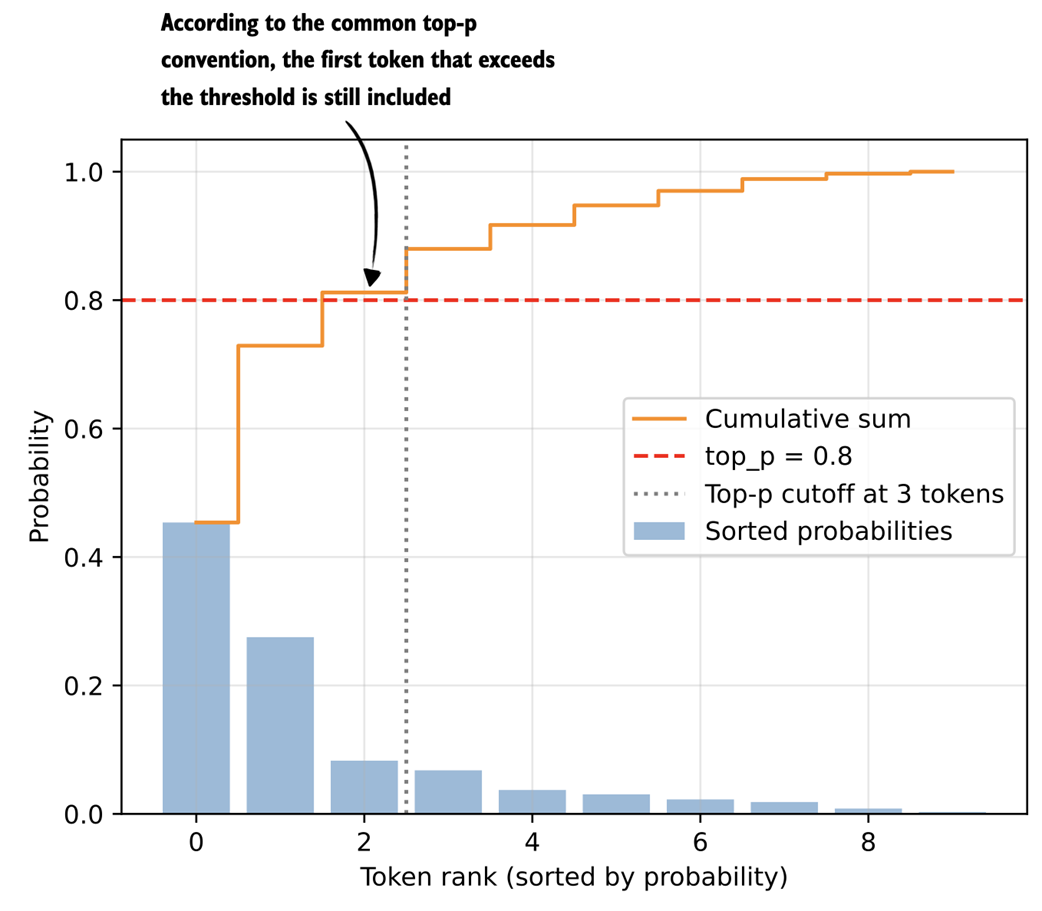 Figure 4.15 Illustration of top-p (nucleus) filtering. Tokens are sorted by probability, and the smallest subset whose cumulative probability exceeds the threshold (p = 0.8) is kept for sampling.
The plot in figure 4.15 shows the top_p = 0.8 threshold value (dashed horizontal line) that defines which tokens are kept. In this case, the cumulative sum of the first two tokens is below the threshold, hence we exclude all other tokens to the right of the cut-off (vertical dotted line).
To implement this threshold cutoff, we can use the following code, which first zeroes out all values to the right side of the cutoff (vertical dashed line in figure 4.15) and restores the original sorting order.
Listing 4.14 Applying top-p filtering
kept_sorted = torch.where(
    keep_mask, sorted_probas,
    torch.zeros_like(sorted_probas)
)
filtered = torch.zeros_like(toy_probas).scatter(0, sorted_idx, kept_sorted)
print(filtered)
The resulting tensor looks as follows:
tensor([0.0000, 0.0000, 0.0000, 0.0000, 0.4538, 0.0000, 0.0000, 0.0000, 0.0829, 0.2752])
We can see that all values except the ones at index positions 4, 8 and 9 are zeroed out. This means that if we now use the multinomial function only those three tokens will be considered. Finally, we renormalize these values so that they sum up to one again:
denom = torch.sum(filtered).clamp_min(1e-12)
renormalized = filtered / denom
print(renormalized)
The resulting, normalized tensor is:
tensor([0.0000, 0.0000, 0.0000, 0.0000, 0.5589, 0.0000, 0.0000, 0.0000,
0.1021, 0.3390])
The goal of top-p filtering, which we implemented in this section, is to remove tokens with low probabilities to avoid them from being sampled later. This helps reduce nonsensical token responses in given contexts.
4.5.2 Adding a top-p filter to the text generation function
In the previous section, we walked through the top-p filtering steps using a simple toy example with a vocabulary size 10 to be able to visualize the procedure in a bar plot. In this section, we are adding the four main top-p filtering steps (steps 4.1-4.4 in figure 4.16) to the existing text generation function.
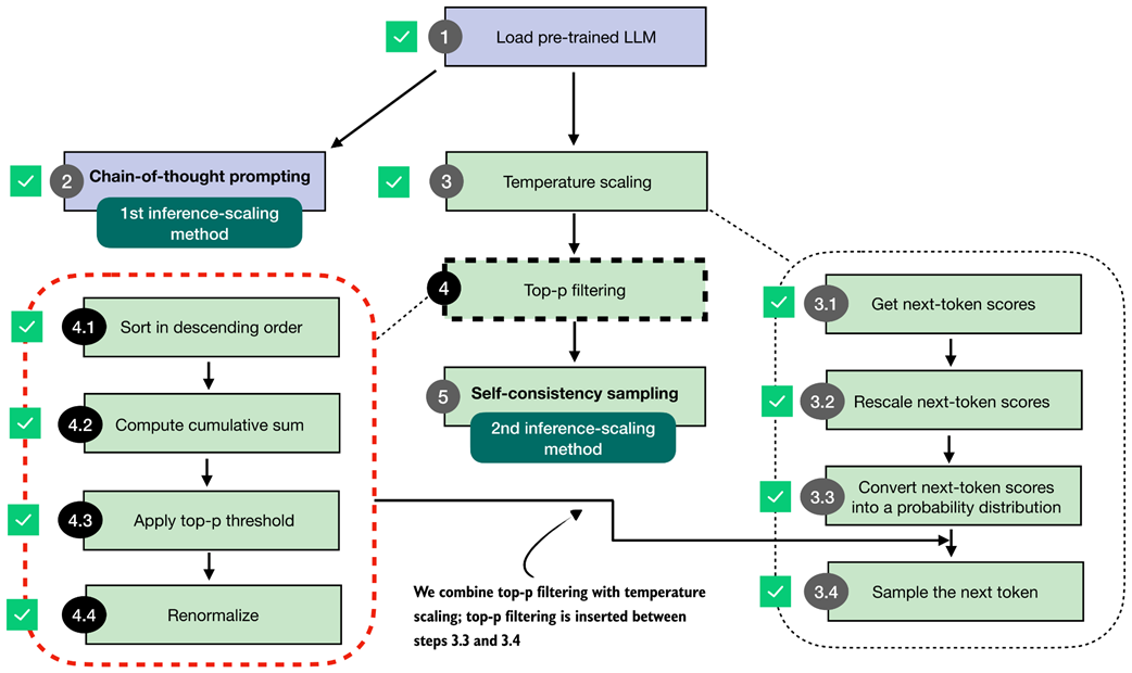 Figure 4.16 Integration of top-p filtering with temperature scaling. After rescaling the next-token scores, top-p filtering is applied between steps 3.3 and 3.4 to limit sampling to the most probable tokens.
Given our previous text generation function, as illustrated in figure 4.16, we add the top-p filtering between the probability conversion and the sampling we implemented earlier in the temperature scaling section.
For this, we will first put together the top-p filtering steps from the previous section into a single, convenient function we can call.
Listing 4.15 Top-p filtering function
def top_p_filter(probas, top_p):
    if top_p is None or top_p >= 1.0:
        return probas

    sorted_probas, sorted_idx = torch.sort(probas, dim=1, descending=True)
    cumprobas = torch.cumsum(sorted_probas, dim=1)

    prefix = cumprobas - sorted_probas
    keep = prefix < top_p
    keep[:, 0] = True

    kept_sorted = torch.where(
        keep, sorted_probas,
        torch.zeros_like(sorted_probas)
    )

    filtered = torch.zeros_like(probas).scatter(1, sorted_idx, kept_sorted)


    denom = torch.sum(filtered, dim=1, keepdim=True).clamp_min(1e-12)
    return filtered / denom
To briefly recap what’s happening in top-p filtering, the top_p_filter function in listing 4.15 first sorts token probabilities and computes their cumulative sum. It then keeps tokens whose prefix cumulative mass (the cumulative probability before each token) is below the top_p threshold, which includes the token that first crosses the threshold. It zeroes out the rest, maps the kept values back to their original order, and renormalizes the remaining probabilities so they sum to 1 again.
Before we add this top_p_filter function to our text generation functions, let’s give it a try and see how it works with the previous temperature-scaling approach. First, we get the logits:
with torch.inference_mode():
    next_token_logits = model(input_token_ids)[:, -1]
print(next_token_logits.shape)
The code above prints the dimensions [1, 151936] for the next_token_logits tensor, since we are now working with the real data and full vocabulary, which has 151,936 entries.
Next, we rescale the logits into probability scores and apply the temperature scaling with a temperature of 0.35, similar to before:
torch.manual_seed(123)
probas_lowT = torch.softmax(
    scale_logits_by_temperature(next_token_logits, 0.35), dim=-1
)
count_samples(probas_lowT, threshold=1, tokenizer=tokenizer)
This code is, so far, similar to what we used in the previous temperature scaling examples and prints the following sampled outputs:
' __': 158x
' Berlin': 435x
' ____': 169x
' ______': 209x
' Munich': 3x
' Hamburg': 3x
' _____': 18x
Now, let’s add the top-p filter and see how it changes the results:
torch.manual_seed(123)
probas_lowT = torch.softmax(
    scale_logits_by_temperature(next_token_logits, 0.35), dim=-1
)
probas_lowT_filtered = top_p_filter(probas_lowT, top_p=0.8)
count_samples(probas_lowT_filtered, threshold=1, tokenizer=tokenizer)
With a top_p threshold of 0.8, which is a typical value, we get rid of the 20% lowest probability tokens, and the sampled outputs now look as follows:
' Berlin': 534x
' ____': 217x
' ______': 249x
As we can see, we now either select the correct city (and remove " Munich" and " Hamburg" as sampled options) or print the underscored token, which the model might use to format the text as a quiz question with the ' ______' as a placeholder.
Now that we walked through the top-p filtering process using a simple toy example, let’s return to our math query and add the top-p filter to the generate_text_temp_stream_cache function we coded earlier. The updated function, now called generate_text_top_p_stream_cache, is shown in listing 4.16 below.
Listing 4.16 Text generation with top-p filtering
@torch.inference_mode()
def generate_text_top_p_stream_cache(
    model,
    token_ids,
    max_new_tokens,
    eos_token_id=None,
    temperature=0.,
    top_p=None
):
    model.eval()
    cache = KVCache(n_layers=model.cfg["n_layers"])
    model.reset_kv_cache()

    out = model(token_ids, cache=cache)[:, -1]
    for _ in range(max_new_tokens):

        orig_device = token_ids.device

        if temperature is None or temperature == 0.0:
            next_token = torch.argmax(out, dim=-1, keepdim=True)

        else:
            logits = scale_logits_by_temperature(out, temperature)
            probas = torch.softmax(logits, dim=-1)

            probas = top_p_filter(probas, top_p)

            next_token = torch.multinomial(probas.cpu(), num_samples=1)
            next_token = next_token.to(orig_device)

        if (eos_token_id is not None
                and torch.all(next_token == eos_token_id)):
            break

        yield next_token
        out = model(next_token, cache=cache)[:, -1]
To conclude this section, let’s plug this new text generation function into the generate_text_stream_concat_flex, similar to what we have done with the temperature-scaling version of the text generation function before:
torch.manual_seed(123)
response = generate_text_stream_concat_flex(
    model, tokenizer, prompt, device,
    max_new_tokens=2048, verbose=True,
    generate_func=generate_text_top_p_stream_cache,
    temperature=0.5,
    top_p=0.8,
)
The output is " \boxed{18}", which is still not correct. However, note that everything we have done up to this point is mainly for the purpose of being able to sample different outputs. In the next section, we will use the generate_text_stream_concat_flex with our augmented text generation function (generate_text_top_p_stream_cache) to sample different outputs when implementing the self-consistency inference-time scaling technique.
Top-k filtering
Top-k filtering is another way to limit the set of candidate next tokens during sampling.
Instead of keeping all tokens whose cumulative probability stays below a threshold (as in top-p), top-k keeps only the k most likely tokens based on the model’s logits.
After sorting the vocabulary by probability, everything past the first k entries is removed.
The remaining k tokens are then renormalized and sampled from.
In short, top-k keeps a fixed number of the most likely tokens, whereas top-p keeps a variable number of tokens depending on their cumulative mass.
Top-k is simpler to implement, and I covered it in my Build a Large Language Model (From Scratch) book. However, top-p sampling has become more popular recently.
Exercise 4.2: Use temperature scaling and top-p filtering on MATH-500
Modify the
evaluate_math500_streamfunction in section 3.9 of chapter 3 to see if adding temperature scaling and top p sampling changes the MATH-500 accuracy of the base model. You can use a setting of 0.9 for both temperature scaling and top-p.
4.6 Improving response accuracy with self-consistency
After all the previous work on coding temperature scaling and top-p filtering, we are now ready to implement the second inference-time scaling technique in this chapter: self-consistency sampling.
The idea behind self-consistency sampling was formally introduced in the Google Research paper Self-Consistency Improves Chain-of-Thought Reasoning in Language Models (https://arxiv.org/abs/2203.11171). However, despite the fancy name, it’s essentially a form of simple majority voting, where we use temperature scaling and top-p filtering to generate multiple answers and then select the most frequent one, as shown in figure 4.17.
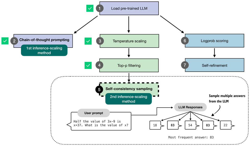 Figure 4.17 The self-consistency sampling method generates multiple responses from the LLM and selects the most frequent answer, which improves answer accuracy through majority voting across these sampled responses.
The self-consistency sampling technique shown in figure 4.17 counts as an inference-time scaling technique, since we don’t update the model itself and we expend more compute resources to improve response accuracy (more on the accuracy later, after we implement and try this technique).
The self-consistency code implementation, thanks to the generate_text_stream_concat_flex function, is relatively straightforward, and the main procedure can be summarized in three main steps as illustrated in figure 4.18.
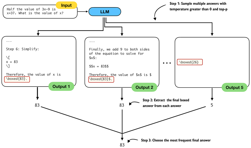 Figure 4.18 The three main steps for implementing self-consistency sampling. First, we generate multiple answers for the same prompt using a temperature greater than zero and top-p filtering to generate different answers. Second, we extract the final boxed answer from each generated solution. Third, we select the most frequently extracted answer as the final prediction.
To implement the three steps illustrated in figure 4.18, in listing 4.15 below, we are simply calling generate_text_stream_concat_flex repeatedly to generate multiple answers and reuse the extract_final_candidate function from chapter 3. The only new code is the majority voting based on the answer frequency.
Listing 4.17 Text generation with top-p filtering
from reasoning_from_scratch.ch03 import extract_final_candidate
from collections import Counter

def self_consistency_vote(
    model, tokenizer, prompt, device,
    num_samples=10, temperature=0.8, top_p=0.9, max_new_tokens=2048,
    show_progress=True, show_long_answer=False, seed=None,
):
    full_answers, short_answers = [], []

    for i in range(num_samples):
        if seed is not None:
            torch.manual_seed(seed + i + 1)

        answer = generate_text_stream_concat_flex(
            model=model, tokenizer=tokenizer, prompt=prompt, device=device,
            max_new_tokens=max_new_tokens, verbose=show_long_answer,
            generate_func=generate_text_top_p_stream_cache,
            temperature=temperature, top_p=top_p,
        )

        short = extract_final_candidate(
            answer, fallback="number_then_full"
        )
        full_answers.append(answer)
        short_answers.append(short)
        if show_progress:
            print(f"[Sample {i+1}/{num_samples}] → {short!r}")

    counts = Counter(short_answers)
    groups = {s: [] for s in counts}
    for idx, s in enumerate(short_answers):
        groups[s].append(idx)

    mc = counts.most_common()
    if not mc:
        majority_winners, final_answer = [], None
    else:
        top_freq = mc[0][1]
        majority_winners = [s for s, f in mc if f == top_freq]
        final_answer = mc[0][0] if len(majority_winners) == 1 else None

    return {
        "full_answers": full_answers,
        "short_answers": short_answers,
        "counts": dict(counts),
        "groups": groups,
        "majority_winners": majority_winners,
        "final_answer": final_answer,
    }
In short, the self-consistency method in listing 4.16 above
- Samples multiple answers with temperature greater than 0 and top-p
- Extracts the final boxed answer from each answer
- Chooses the most frequent final answer
Note that in our implementation, we use a for-loop to generate these answers sequentially. In practice, it is also common to generate the answers on different devices so that the sampling can be parallelized.
Furthermore, in the code above, we set the random seed for each round individually:
if seed is not None:
            torch.manual_seed(seed + i + 1)
Technically, this is not necessary and setting the random seed once should be sufficient to generate diverse samples. However, this explicit seeding is useful if we want to individually rerun some of the rounds.
Let’s try out this function in practice and see what we get:
results = self_consistency_vote(
    model,
    tokenizer,
    prompt,
    device=device,
    num_samples=5,
    temperature=0.8,
    top_p=0.9,
    max_new_tokens=2048,
    seed=123,
    show_progress=True,
)
The printed results are shown below:
[Sample 1/5] → '83'
[Sample 2/5] → '22'
[Sample 3/5] → '54'
[Sample 4/5] → '83'
[Sample 5/5] → '61'
The top final answer, since 83 is the most frequent answer, is 83 (we can access this number programmatically via results["final_answer"]). If you want to read the explanation and full answer, you can access one of the correct solutions returning 83, for example print(results["full_answers"][0]), which prints:
To find the value of x, let's solve the equation step by step.

1. **Given Equation:**
   \[
   \frac{1}{2} \times (3x - 9) = x + 37
   \]

# ...

**Final Answer:**
\[
\boxed{83}
\]
Finally, with this self-consistency approach, we were able to generate the correct answer. (Note that the results may vary when executing the code on an "mps" or "cuda" device.)
The self_consistency_vote function currently also does not handle ties, so if multiple samples have the same frequency, it returns None as the final answer. We will implement a scoring method in the next chapter to calculate the confidence of a given answer, which can be used as a tie-breaker.
Exercise 4.3: Use self-consistency sampling on MATH-500
Modify the
evaluate_math500_streamfunction in section 3.9 of chapter 3 to evaluate whether self-consistency sampling improves the MATH-500 accuracy of the base model. Use a sample size of 3 and set both the temperature and top-p value to 0.9.As part of this exercise, implement tie-breaking so that ties are resolved by the first answer appearing in the sample list. For example, if the sampled answers are 13, 15, 13, 15, 16, the selected answer should be 13.
Note that you don’t have to modify the
self_consistency_voteitself to implement this tie-breaking, but you can work with theresultsdictionary returned by the function to implement this simple tie-breaking rule.
Exercise 4.4: Early stopping in self-consistency sampling
To improve computational efficiency, implement an early-stopping version of self-consistency that ends sampling once more than half of the answers agree.
Choosing temperature and top-p settings
For reasonable results, temperature settings are usually between 0.5 and 0.9, and a top-p value of 0.7 to 0.9 is typical.
As a rule of thumb, if all (long) answers look nearly identical, it’s a good idea to increase the temperature gently to increase diversity. Here, “long” answer means the full answer before extracting the final boxed result. You can inspect the long answers in the results dictionary returned by the self_consistency_vote function or run the function with the
show_long_answer=Truesetting.If (long) answers look off or nonsensical, it usually means the temperature is too high and should be decreased.
You may recall that the aforementioned paper title that described this technique was Self-Consistency Improves Chain-of-Thought Reasoning in Language Models. Where or how does the “chain-of-thought reasoning” aspect factor into all of this?
Chain-of-thought reasoning here simply refers to the chain-of-thought prompting we introduced earlier in this chapter, when we modified the prompt via "\n\n Explain step by step." so that the LLM generates longer responses.
So, let’s combine chain-of-thought prompting with self-consistency sampling:
results = self_consistency_vote(
    model,
    tokenizer,
    prompt + "\n\nExplain step by step.",
    device=device,
    num_samples=5,
    temperature=0.8,

    top_p=0.9,
    max_new_tokens=2048,
    seed=123,
    show_progress=True,
)
In this case, all 5 answers are 83 (correct), likely because the question is relatively simple for the LLM when using a chain-of-thought.
Instead, it would be more interesting to see how well the model performs on the entire MATH-500 dataset from the previous chapter. The results from various experiments are shown in table 4.1.
Table 4.1 MATH-500 task accuracy for different methods
| # | Method | Model | Accuracy | Time |
|---|---|---|---|---|
| 1 | Baseline (chapter 3), greedy decoding | Base | 15.2% | 10.1 min |
| 2 | Baseline (chapter 3), greedy decoding | Reasoning | 48.2% | 182.1 min |
| 3 | Chain-of-thought prompting (“CoT”) | Base | 40.6% | 84.5 min |
| 4 | Temperature and top-p (“Top-p”) | Base | 17.8% | 30.7 min |
| 5 | “Top-p” + Self-consistency (n=3) | Base | 29.6% | 97.6 min |
| 6 | “Top-p” + Self-consistency (n=5) | Base | 27.8% | 116.8 min |
| 7 | “Top-p” + Self-consistency (n=10) | Base | 31.6% | 300.4 min |
| 8 | “Top-p” + “CoT” | Base | 33.4% | 129.2 min |
| 9 | Self-consistency (n=3) + “Top-p” + “CoT” | Base | 42.2% | 211.6 min |
| 10 | Self-consistency (n=5) + “Top-p” + “CoT” | Base | 48.0% | 452.9 min |
| 11 | Self-consistency (n=10) + “Top-p” + “CoT” | Base | 52.0% | 862.6 min |
| 12 | Self-consistency (n=3) + “Top-p” + “CoT” | Reasoning | 55.2% | 544.4 min |
The accuracy values shown in table 4.1 were computed on all 500 samples in the MATH-500 test set using a “cuda” GPU (RTX 4090). Let’s go through the results one by one. The n=3 abbreviation means that we used a sample size of 3 in self-consistency sampling.
Rows 1 and 2 show the results of the base and reasoning variants using the code from chapter 3, meaning we use the text generation function without temperature scaling or top-p filtering. This text function simply selects the token with the highest score at each step, which is also known as greedy decoding. We can see that the reasoning variant has approximately 3 times the accuracy but also substantially increased runtime, since it generates more tokens.
Next, in row 3, we see the results for the chain-of-thought prompting approach via the "\n\nExplain step by step." prompt modification. As we can see, this boosts the base model’s accuracy from approximately 15% to 40%.
Row 4 shows what happens when we add temperature-scaling and top-p sampling to the base model. (All experiments involving temperature scaling and top-p sampling in table 4.1 used a setting of 0.9 for both.) As we can see, the accuracy over the base model row 1 is only moderately improved from 15.2% to 17.8%. This is expected because temperature-scaling and top-p scaling merely help us to control the sampling diversity but are not inference-time scaling techniques themselves. We can also see that the runtime increased from 10.1 min to 30.7 min. This is not due to the sampling code overhead, but rather because the model now generates longer responses in some cases.
Rows 5-7 show the self-consistency scaling results. We can see that increasing the number of samples from 3 to 10 further improves accuracy to 31.6%, but it also significantly increases runtime. In this case, there is almost no accuracy advantage to using 10 instead of 3 samples.
Row 8 shows temperature-scaling and top-p sampling combined with chain-of-thought prompting. In this case, the sampling makes the chain-of-thought results worse (33.4% compared to the 40.6% in row 3). However, when combining chain-of-thought prompting with self-consistency, we can see that accuracy improves to 52% with a sample size of 10, but this also substantially increases runtime to a staggering 862.9 min.
However, note that in practice, if you have access to multiple GPUs, the different samples in self-consistency sampling can be computed in parallel rather than sequentially. This would still use the same amount of compute, but it could be distributed and parallelized to generate the results faster.
Lastly, in row 12, we can see that the reasoning variant benefits from self-consistency sampling as well, taking the performance of the reasoning variant (row 2) from 48.2% to 55.2% accuracy. Again, this comes at an increased runtime.
The takeaway is that the results in table 4.1 nicely highlight the trade-off in inference-time scaling, where we trade better accuracy for more compute.
Note that one major downside of the self-consistency sampling approach in this chapter is that it relies on a final boxed answer that we can extract for majority voting. This method is trickier to apply to problems that don’t have numeric or short final answers.
In the next chapter, as illustrated in figure 4.19, we will implement a different and more versatile inference-time scaling method called self-refinement, in which the model iteratively improves its own answers.
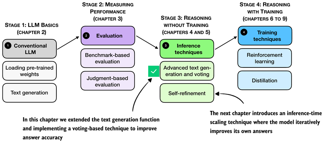 Figure 4.19 Summary of this chapter’s focus on inference-time techniques. Here, the text generation function was extended with a voting-based method to improve answer accuracy. The next chapter introduces self-refinement, in which the model iteratively improves its responses.
4.7 Summary
- Reasoning abilities and answer accuracy can be improved without retraining the model by increasing compute at inference time (inference-time scaling).
- This chapter focuses on two such techniques: chain-of-thought prompting and self-consistency; a third method, self-refinement, which was briefly described, will be covered in for the next chapter.
- A flexible text generation wrapper (
generate_text_stream_concat_flex) that uses different sampling strategies that can be plugged in without changing the surrounding code. - Next tokens are produced from logits via softmax
- Temperature scaling changes logits to control the diversity of the generated text.
- Top-p (nucleus) sampling filters out low-probability tokens to reduce the chance of generating nonsensical answers
- Chain-of-thought prompting (like “Explain step by step.” or similar) often yields more accurate answers by encouraging the model to write out intermediate reasoning, though it increases the number of generated tokens and thus increases the runtime cost.
- Self-consistency sampling generates multiple answers, extracts the final boxed result from each, and selects the most frequent answer via majority vote to improve the answer accuracy.
- Experiments on the MATH-500 dataset show that combining chain-of-thought prompting with self-consistency can substantially boost accuracy compared to the baseline without sampling, at the cost of much longer runtimes.
- The central trade-off of inference-time scaling: higher accuracy in exchange for more compute.