7 Improving GRPO for reinforcement learning

This chapter covers

• Interpreting training curves and evaluation metrics
• Preventing the model from exploiting the reward signal
• Extending task-correctness rewards with additional response-formatting rewards

Previously, we implemented the GRPO algorithm for reinforcement learning with verifiable rewards (RLVR) end to end. Now, as shown in figure 7.1, we pick up from that baseline and focus on what happens when we run longer training.

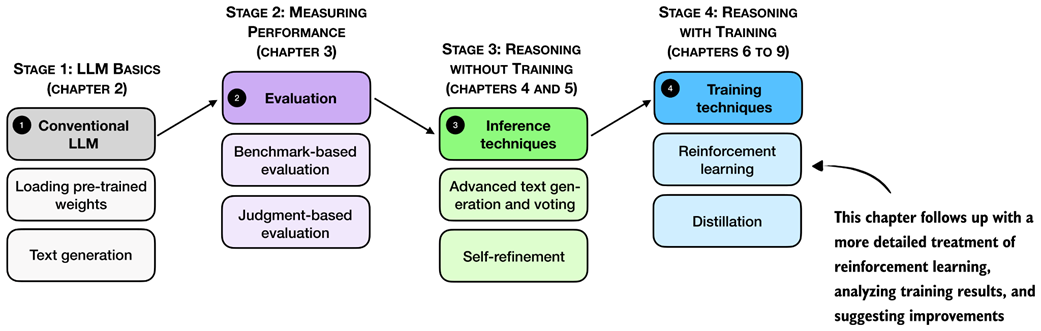Figure 7.1 A mental model of the topics covered in this book. This chapter provides a deeper coverage of the GRPO algorithm for reinforcement learning with verifiable rewards.

In particular, we will discuss which metrics are worth tracking (beyond reward and accuracy), how to spot failure modes early, and why training can become unstable even when the code is “correct.” We then introduce practical GRPO extensions and fixes used in reasoning-model training.

7.1 Improving GRPO

After implementing GRPO (group relative policy optimization) in the previous chapter, we now revisit and analyze the training run more thoroughly. Also, we discuss a collection of practical tips and algorithmic choices that become important in real training runs. These topics are summarized in the chapter overview in figure 7.2.

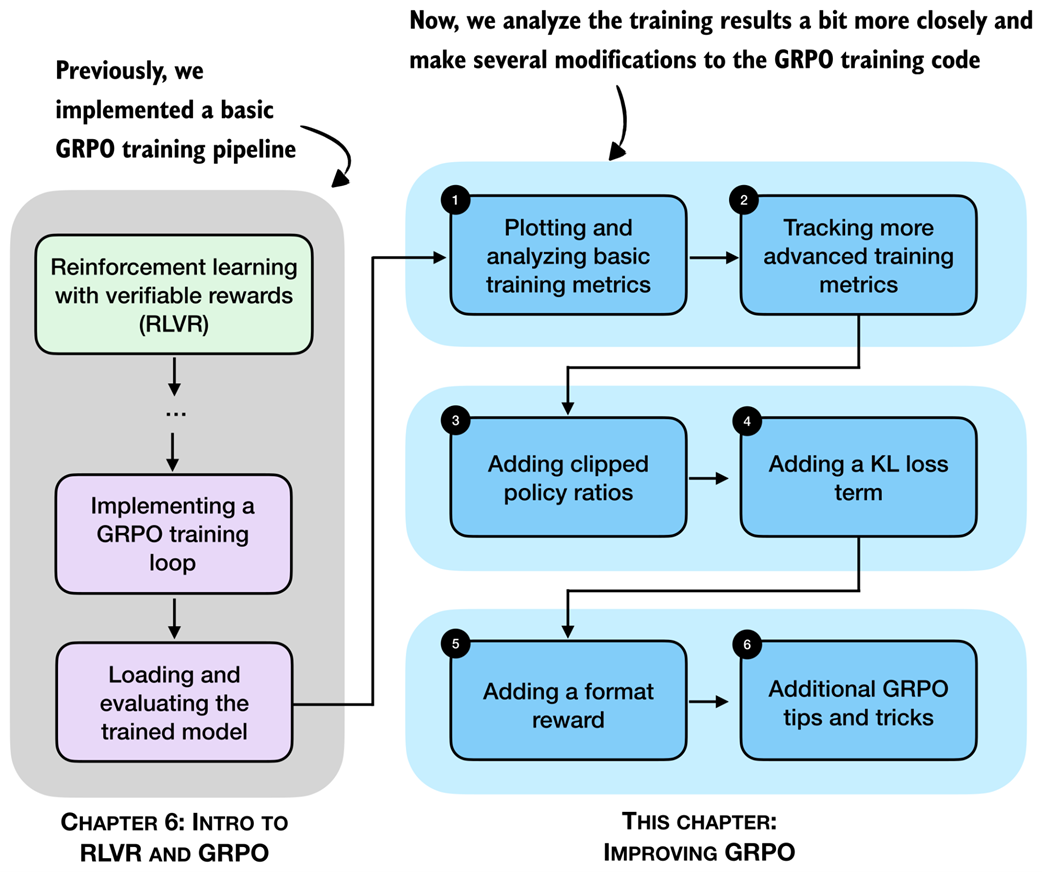Figure 7.2 A chapter overview showing the different topics being covered in this chapter.

The examples in this chapter are based on actual experiments, but the results should be interpreted with care. To draw strong conclusions about the effect of individual settings, each experiment would need to be repeated multiple times and the results averaged, since randomness in sampling and optimization can lead to noticeable variation between runs. That said, the examples shown here are sufficient to illustrate the main ideas and the relevant trade-offs.

Note

This chapter focuses on additional technical details and practical considerations when using GRPO. Readers who find the content in this chapter too technical and prefer to move on can do so, as the next chapter does not depend on it.

7.2 Tracking GRPO performance metrics

In chapter 6, we ran a short GRPO training loop and briefly examined the results. For example, the output of a short run was structured as follows:

[Step 1/50] loss=-0.0000 reward_avg=0.000 avg_resp_len=5.5
[Step 2/50] loss=-0.0000 reward_avg=0.000 avg_resp_len=6.8
[Step 3/50] loss=0.3592 reward_avg=0.250 avg_resp_len=7.8
[Step 4/50] loss=2.7401 reward_avg=0.250 avg_resp_len=56.5
[Step 5/50] loss=3.3214 reward_avg=0.500 avg_resp_len=251.2
# ...

Let’s pick up from this point and discuss which metrics to track when training with GRPO, and how they help interpret and debug training behavior.

7.2.1 Executing a GRPO training run

The code in chapter 6 is designed to strike a balance between implementing the complete GRPO pipeline and keeping the implementation compact enough to remain readable. For convenience, the supplementary materials include an equivalent script (https://github.com/rasbt/reasoning-from-scratch/blob/main/ch06/02_rlvr_grpo_scripts_intro/rlvr_grpo_original_no_kl.py), which contains the same code and can be run from a code terminal (more on this later).

For each GRPO improvement introduced, we will use similar reference scripts from the supplementary materials to avoid duplicating large code blocks that would otherwise unnecessarily bloat the chapter and the surrounding discussion.

Using the helper function in listing 7.1, we can download the relevant scripts from the supplementary materials and save them locally as needed throughout this chapter.

Listing 7.1 Helper function to download supplementary materials

from pathlib import Path
import requests
 
def download_from_github(rel_path, out=None):
    github_raw_base = (
        "https://raw.githubusercontent.com/rasbt/"
        "reasoning-from-scratch/refs/heads/main/"
    ) # A
 
    rel_path = Path(rel_path)

    out = Path(out) if out is not None else Path(rel_path.name) # B
 
    if out.exists():
        size_kb = out.stat().st_size / 1e3
        print(f"{out}: {size_kb:.1f} KB (cached)")
        return out # C
 

    r = requests.get(github_raw_base + rel_path.as_posix())
    r.raise_for_status()
 
    out.write_bytes(r.content)
    size_kb = out.stat().st_size / 1e3
    print(f"{out}: {size_kb:.1f} KB") # D

• A: Base URL
• B: Use URL file name as default output file name
• C: Skip download if file already exists locally
• D: Download file

Using the helper function, we can download the aforementioned script with the GRPO training code from chapter 6 as follows:

download_from_github(
    "ch06/02_rlvr_grpo_scripts_intro/rlvr_grpo_original_no_kl.py"
)

When executing the code above, you should see the following output: rlvr_grpo_original_no_kl.py: 13.4 KB

If the downloaded files are much smaller than the sizes shown above, the download may not have completed correctly. In that case, first double-check that the URLs don’t have any typos. If the problem persists, please check the troubleshooting guide (https://github.com/rasbt/reasoning-from-scratch/blob/main/troubleshooting.md) for additional suggestions.

The resulting script can be run from a terminal as shown in figure 7.3.

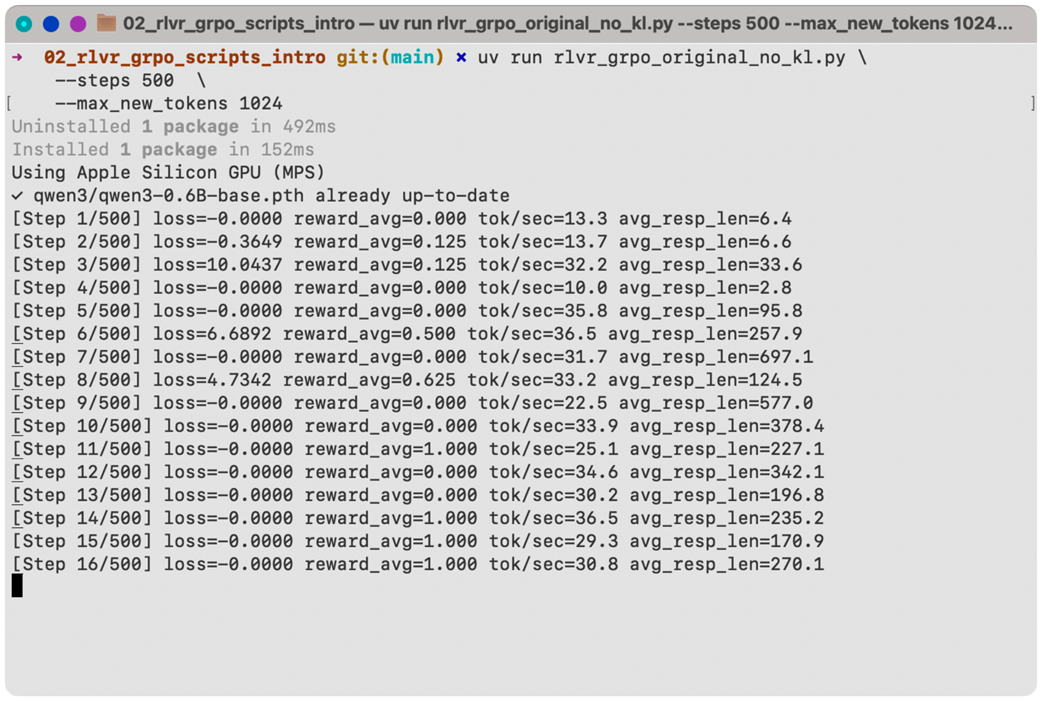Figure 7.3 Output from a GRPO training run using GRPO in a terminal with several training statistics, such as the loss, average reward, tokens/sec throughput, and average response length.

It’s also possible to run the training script in Jupyter notebooks in a code cell by prepending an !, i.e., !uv run rlvr_grpo_original_no_kl.py.

If you are not a uv user, replace uv run shown in figure 7.3 with python, that is, python rlvr_grpo_original_no_kl.py:

python rlvr_grpo_original_no_kl.py \
--steps 500  \
--max_new_tokens 1024

If you prefer not to run the training code yourself, which is reasonable given its computational cost, the supplementary materials provide log files from this run. We can download these as follows:

download_from_github(
"ch06/02_rlvr_grpo_scripts_intro/logs/"
"rlvr_grpo_original_no_kl_metrics.txt"
)
download_from_github(
"ch06/02_rlvr_grpo_scripts_intro/logs/"
"rlvr_grpo_original_no_kl_metrics.csv"
)

The first file, ending in .txt, is the plain output file that shows the output statistics similar to figure 7.3. The second file, ending in .csv, is a comma-separated values file that provides more structure to this information so that we can more easily extract and plot the data for further analysis.

7.2.2 Inspecting the GRPO training run

To inspect the training run, we plot the results from the previous log files using Matplotlib. For this, we define the following plotting function that we will use throughout this chapter:

Listing 7.2 Plotting function to visualize training results from log files

import csv
import matplotlib.pyplot as plt
 
 
def moving_average(values, window_fraction=0.25): # A

    window_size = max(1, int(window_fraction * len(values)))
    smoothed = []
 
    for i in range(len(values)):
        start_idx = max(0, i - window_size + 1)
        window_mean = sum(values[start_idx : i + 1]) / (i - start_idx + 1)
        smoothed.append(window_mean)
 
    return smoothed
 
 
def plot_grpo_metrics(csv_path, columns, save_as=None):
    data = {name: {"steps": [], "values": []} for name in columns}
 
    with Path(csv_path).open(newline="") as f: # B
        reader = csv.DictReader(f)
        for row in reader:
            if not row or not row.get("step"):
                continue
            
            step = int(row["step"])
 
            for name in columns:
                value_str = row.get(name)
                if value_str:
                    data[name]["steps"].append(step) # C
                    data[name]["values"].append(float(value_str))
 

    fig, axes = plt.subplots(2, 2, sharex=True, figsize=(6, 4)) # D
    axes = axes.ravel()
 
    for i, name in enumerate(columns):
        steps = data[name]["steps"]
        values = data[name]["values"]
 
        if not values:
            fig.delaxes(axes[i])
            continue # E
 
        if name == "eval_acc":
            axes[i].bar(steps, values, width=20) # F
        else:
            axes[i].plot(steps, values, alpha=0.4)
            axes[i].plot(steps, moving_average(values))
 
        axes[i].set_ylabel(name)
 
    for j in (2, 3):
        if axes[j] in fig.axes:
            axes[j].set_xlabel("Step")
 
    plt.tight_layout()
    if save_as is not None:
        plt.savefig(save_as)
    plt.show()

• A: Smooth the noisy training signal to reveal longer-term trends during training
• B: Open and read CSV log file
• C: Use the training step as the shared x-axis across all metrics
• D: Create a fixed grid so loss, rewards, response length, etc. can be shown side by side
• E: Skip metrics that are not present
• F: Evaluation accuracy as barplot because we don’t have data for each step

The .csv file we downloaded has multiple columns. Using the plot_grpo_metrics function we defined in listing 7.2, we plot the loss, average reward, average response length, and evaluation accuracy:

plot_grpo_metrics(
    "rlvr_grpo_original_no_kl_metrics.csv",
    columns=["loss", "reward_avg", "avg_response_len", "eval_acc"]
)

The resulting plot is shown in figure 7.4.

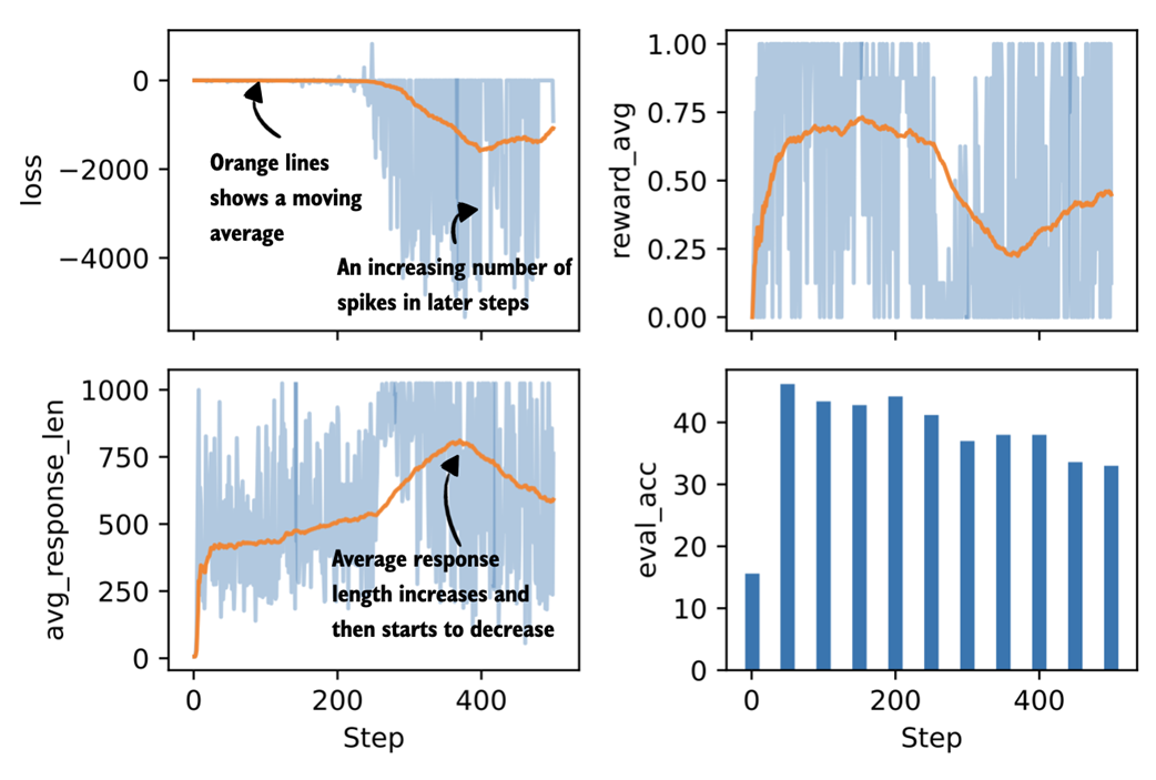Figure 7.4 Plots visualizing four metrics tracked during the GRPO training run (loss, average reward, average response length, and evaluation accuracy). The orange centerline represents a moving average over the last 25% of values, which helps reveal overall trends in the otherwise noisy training signals. The evaluation accuracy is shown as a bar plot since it is computed only every 50 steps rather than at each step.

A few general observations stand out in the plots shown in figure 7.4. The average response length should initially increase, ideally together with an improvement in accuracy, which is largely what we see here, although there is a noticeable decline later in the run just before step 400. Compared to LLM pre-training, which is outside the scope of this book and covered in more detail in Build a Large Language Model (From Scratch), the loss value itself is less informative and mainly serves as a sanity check. Overall, the loss should remain relatively stable. Some fluctuations are expected, but the larger spikes that appear halfway through the run are a bit concerning.

The average reward should also increase over time. In principle, an average reward of 1.00 means that all sampled responses are correct, which is desirable, but it also means that the training signal has disappeared. At that point, further training is unlikely to be useful, and stopping early can save us time and resources.

Finally, performance on the external target task, here measured by MATH-500 accuracy, should improve. In this run, accuracy increases at first but then begins to decline, which points to problems and instabilities in the training process.

In summary, the training run shows fast gains early on and is followed by diminishing returns after approximately fifty steps. One likely reason is that the underlying algorithm is not particularly stable over longer runs. Another possible explanation could be that later training examples are more difficult, but this would not account for decline in evaluation accuracy, which is computed from the same 500 MATH-500 test samples every fifty steps.

Note that the main goal of this section is to introduce, analyze, and discuss various training metrics. This section focused on some basic ones, and in the next section, we will extend this list and look at additional metrics that are commonly tracked during GRPO training.

Calculating the evaluation accuracy

Evaluation accuracy (eval_acc), here measured on the MATH-500 benchmark, is not tracked by default during training. It can be computed periodically by adding the setting --eval_every_steps 500 when running the training script. However, this is not recommended as this significantly slows down training. Alternatively, it can be calculated separately after training using the evaluate_math500.py script introduced in chapter 3:

download_from_github(
    "ch03/02_math500-verifier-scripts/evaluate_math500.py"
)

The evaluation can then be run as follows on a given checkpoint:

uv run evaluate_math500.py \
  --dataset_size 500 \
  --checkpoint_path \
    "checkpoints/rlvr_grpo_original_no_kl/\
qwen3-0.6B-rlvr-grpo-step00050.pth"

In the run discussed above, evaluation accuracy is already included in the log file.

7.3 Tracking more advanced GRPO performance metrics

Beyond the small set of basic metrics for monitoring GRPO training runs, there are several additional ones that can be useful for understanding training dynamics, as illustrated in figure 7.5.

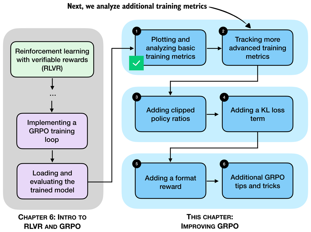Figure 7.5 After analyzing basic GRPO training metrics, we now add more advanced metrics to analyze the training run.

Two examples of the more advanced metrics mentioned in figure 7.5 are the rollout advantages already computed in the compute_grpo_loss function from chapter 6, and the entropy of the generated sequences.

7.3.1 Advantage tracking

As part of the GRPO algorithm, we compute so-called advantages, as discussed in chapter 6, and shown in figure 7.6. Beyond their role in the loss computation, these values are also useful for analyzing and understanding training dynamics.

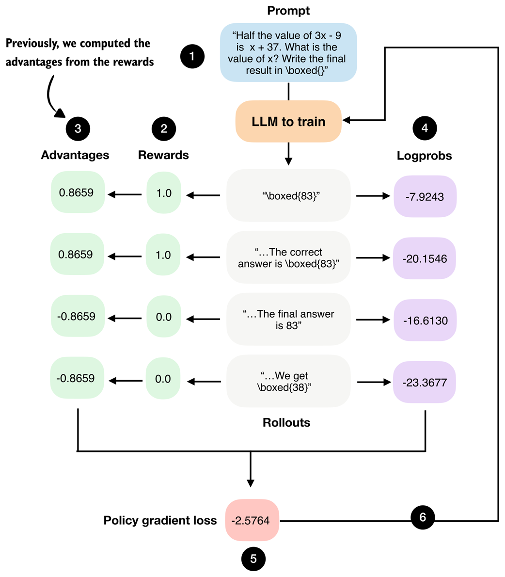Figure 7.6 GRPO overview figure from chapter 6. The advantages are shown in step 3.

In particular, we compute two summary statistics derived from the advantages shown in figure 7.6, namely, their average value (the sample mean) and their standard deviation:

Listing 7.3 Computing advantage statistics

import torch
 
def compute_advantage_stats(rewards_list):

    rewards = torch.tensor(rewards_list)
    advantages = (rewards - rewards.mean()) / (rewards.std() + 1e-4) # A
 

    adv_avg = advantages.mean().item()
    adv_std = advantages.std().item() # B
 
    return advantages, adv_avg, adv_std

• A: The rewards and advantages below are what we already compute in GRPO
• B: Now, we also compute the average (mean) and standard deviation (std)

As a simple illustration, consider a small sample of four reward values, similar to those shown in the previous figure 7.6.

adv, adv_avg, adv_std = compute_advantage_stats([1., 1., 0., 0.])
print(f"Advantages: {adv}")
print(f"Advantage mean = {adv_avg:.4f}, std = {adv_std:.4f}")

The output is:

Advantages: tensor([ 0.8659,  0.8659, -0.8659, -0.8659])
Advantage mean = 0.0000, std = 0.9998

Because of how advantages are computed in GRPO, their mean is always zero. In practice, this makes the mean mostly a sanity check that the implementation behaves as expected.

The standard deviation is more informative. Values close to 1 indicate a well-scaled gradient signal and are usually associated with stable updates. Very small values point to a vanishing learning signal, which often happens when rewards collapse. Very large values indicate overly spiky updates that can destabilize training.

An extreme case occurs when all rewards are identical. When all advantages are identical, which is indicated by a standard deviation that is zero, the policy gradient becomes zero and no model weight update occurs. In other words, the model fails to learn to improve in these cases. For example, consider the following scenario:

adv, adv_avg, adv_std = compute_advantage_stats([0., 0., 0., 0.])
print(f"Advantages: {adv}")
print(f"Advantage mean = {adv_avg:.4f}, std = {adv_std:.4f}")

which prints the following outputs:

Advantages: tensor([0., 0., 0., 0.])
Advantage mean = 0.0000, std = 0.0000

And the outputs are similar if we replace the all-zero rewards in compute_advantage_stats([0., 0., 0., 0.]) with all-one rewards compute_advantage_stats([1., 1., 1., 1.]).

In practice, it is best to consider the advantage statistics together with the average reward. As mentioned earlier, an average reward of 1.0 is actually a desirable outcome, even though it means that the training signal has disappeared because the model is answering everything correctly. At this point, it usually makes sense to stop training or to switch to more challenging examples.

Population versus sample standard deviation

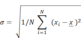
As a side note, please note that PyTorch computes the population standard deviation by default (unbiased=False). For readers with a background in statistics, this corresponds to the standard deviation formula that divides by N:

Here, N is the number of data points in the list or tensor, $x_i$ is a single data point, and $\bar{x}$ is the sample mean (average).

Setting unbiased=True applies Bessel’s correction and divides by N-1 instead.

For example, for the advantages adv = torch.tensor([0.8659, 0.8659, -0.8659, -0.8659]), the population standard deviation via adv.std() is 0.9998, while the sample standard deviation via adv.std(unbiased=True) is 1.1545. This difference is only a constant scaling factor and does not change the qualitative interpretation. In practice, the standard deviation is used as a relative diagnostic for gradient scaling and training stability rather than as a statistical estimator.

7.3.2 Entropy tracking

Before we track and analyze the advantage statistics introduced in the previous section, we introduce another metric to track, entropy.

Entropy measures how uncertain the model is when generating the next token. High entropy means the probabilities are spread across many possible tokens, which encourages exploration. Low entropy means most of the probability is concentrated on a single token, which makes the model increasingly deterministic. It also potentially signals training collapse, where the model stops exploring and keeps producing the same outputs.

Before computing entropy, it is useful to briefly revisit how we calculated log-probability values (logprobs) in chapter 5, as summarized in figure 7.7.

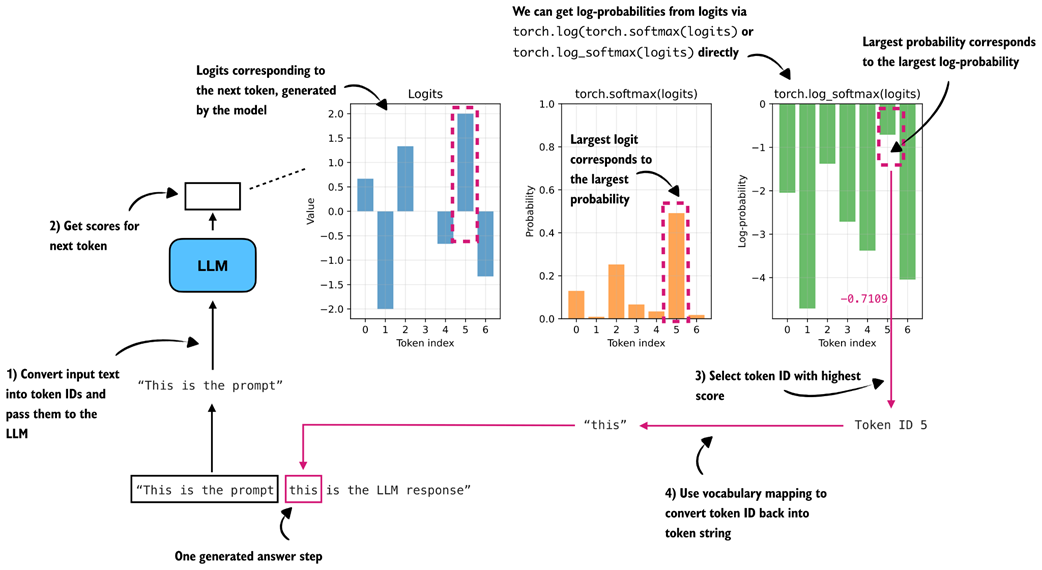Figure 7.7 Log-probability (logprob) computation of a single token ("this") in the LLM’s generated answer. The LLM returns the logits of the token, which are then converted to softmax probability values via torch.softmax() or logprob values via torch.log_softmax().

In figure 7.7, instead of using real logits created by prompting the base model, we use example logits assuming a vocabulary size of 7 (otherwise, with the original 151-thousand-token vocabulary, it would be impossible to visualize this concept in a plot):

logits = torch.tensor([
    0.6667, -2.0000,  1.3333, -0.0000, -0.6667,  2.0000, -1.3333
])

The following code implements the calculation shown in the previous figure 7.7:

logprobs = torch.log_softmax(logits, dim=-1)
print("All token logprobs:", logprobs)
 
selected_token = torch.argmax(logprobs)
selected = logprobs[selected_token]
print("Selected token ID:", selected_token)
print("Selected token logprob:", selected)

The outputs are:

All token logprobs: tensor([-2.0442, -4.7109, -1.3776, 
-2.7109, -3.3776, -0.7109, -4.0442])
Selected token ID: tensor(5)
Selected token logprob: tensor(-0.7109)

In short, the torch.log_softmax() function computes all log-probabilities (logprobs), the torch.argmax() returns the index (token ID) of the largest logprob (here: 5), and the logprobs[selected_token] returns the logprob value of that token ID (-0.7109).

Entropy is closely related to the log-probabilities. We compute it by multiplying each probability by its log-probability and then summing these products, as illustrated in figure 7.8.

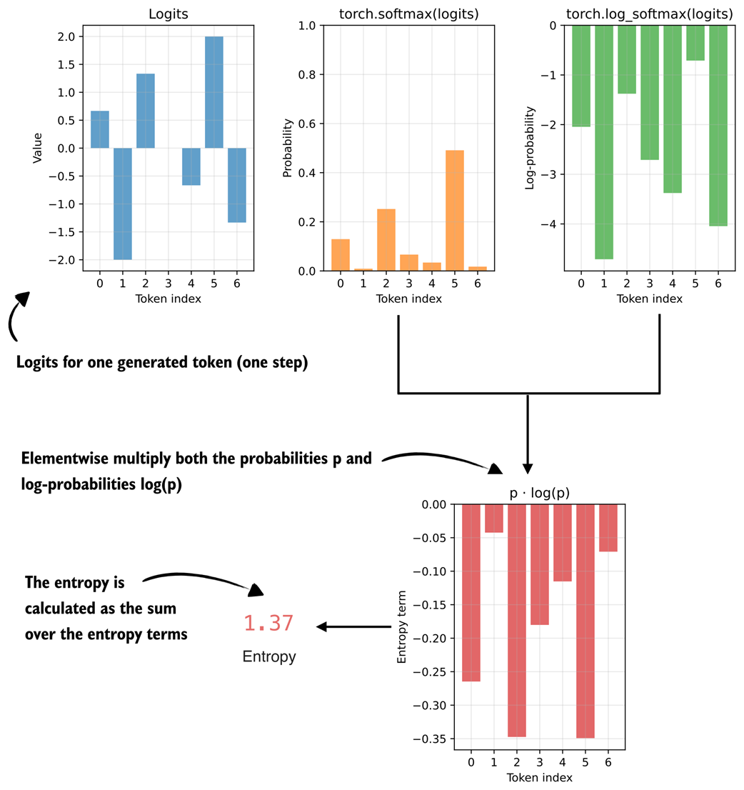Figure 7.8 The entropy term is calculated by multiplying the token probabilities with the token logprobs.

Figure 7.8 shows that the entropy is computed by multiplying probability and logprob values. In principle, we could also track simpler quantities than entropy during training, such as the sum of probabilities or logprobs, but entropy is a widely used and easy-to-interpret measure of uncertainty in a probability distribution.

In the previous figure, we see an entropy of 1.37. As a rough rule of thumb:

• Very low entropy (≈ 0-0.5) means that one token dominates the distribution. The model is highly confident and behaves almost deterministically.
• Moderate entropy (≈ 1-2) means the probabilities are shared across a reasonably small set of tokens, which is typical during stable training.
• High entropy (≫ 2, approaching log(vocabulary size); here: log(7) = 1.9459) means the probabilities are spread across many tokens. In this case, the model is highly uncertain and behaves close to random.

We can calculate the entropy as follows in code:

Listing 7.4 Calculating entropy

probs = torch.softmax(logits, dim=-1)
logprobs = torch.log_softmax(logits, dim=-1)
entropy = torch.sum(-(probs * logprobs))
 
print("Probs:", probs)
print("Entropy:", entropy)

The resulting outputs are:

Probs: tensor([0.1295, 0.0090, 0.2522, 0.0665, 0.0341, 0.4912, 0.0175])
Entropy: tensor(1.3700)

As mentioned earlier, entropy quantifies how spread out the model’s probability distribution is over the vocabulary. In this specific example, the entropy of 1.37 indicates a moderate level of uncertainty. One token (with probability 0.4912) clearly dominates, but other tokens still have meaningful probabilities, too.

Note that in the previous code listing, we compute the probs and logprobs separately using torch.softmax() and torch.log_softmax(), respectively. The torch.log_softmax() function combines two separate function calls: torch.log(torch.softmax()). And the torch.exp() function is the inverse of torch.log(). This means, if we only had the logprobs, we could also calculate the probs by applying torch.exp(logprobs), as follow:

print("Probs:", torch.exp(logprobs))

This outputs the same probs values as before:

Probs: tensor([0.1295, 0.0090, 0.2522, 0.0665, 0.0341, 0.4912, 0.0175])

Building on this idea, we can extend the sequence_logprob function from the previous chapter to a sequence_logprob_and_entropy function that returns both the logprobs and the entropy.

Listing 7.5 Calculating sequence logprob and average entropy

def sequence_logprob_and_entropy(model, token_ids, prompt_len):

    logits = model(token_ids.unsqueeze(0)).squeeze(0).float()
    logprobs = torch.log_softmax(logits, dim=-1)
 
    targets = token_ids[1:]
    selected = logprobs[:-1].gather(1, targets.unsqueeze(-1)).squeeze(-1)
 

    selected_answer_logprobs = selected[prompt_len - 1:]
    logp_all_steps = torch.sum(selected_answer_logprobs) # B
 

    all_answer_logprobs = logprobs[:-1][prompt_len - 1:]
    if all_answer_logprobs.numel() == 0:
        entropy_all_steps = logp_all_steps.new_tensor(0.0) # D
    else:

        all_answer_probs = torch.exp(all_answer_logprobs) # E

        plogp = all_answer_probs * all_answer_logprobs # F

        step_entropy = -torch.sum(plogp, dim=-1) # G

        entropy_all_steps = torch.mean(step_entropy) # H
 
    return logp_all_steps, entropy_all_steps

• A: Code below is identical to the sequence_logprob code in chapter 5
• B: Logprob of the generated answer tokens (sum over answer steps)
• C: Below is the new code that calculates the entropy
• D: A safeguard that is triggered if the model immediately returns EOS token
• E: Convert logprob to prob
• F: Calculate elementwise p * log p
• G: Calculate entropy for single tokens (generation steps) by summing over all plogp values in the vocabulary
• H: Average over all answer steps to calculate average entropy for a given LLM answer

To compute and track the entropy during training, we can use this sequence_logprob_and_entropy function inside compute_grpo_loss in place of the sequence_logprob function.

Note that the previous figure illustrated the entropy computation for a single token in the rollout (step_entropy), whereas sequence_logprob_and_entropy returns the average entropy over all answer tokens, that is, entropy_all_steps = torch.mean(step_entropy). For example, for the answer "this is the LLM response", the step entropy refers to the entropy at a single token position (for instance at "this"), while the average entropy is the mean taken across all answer tokens in "this is the LLM response".

With this modified sequence_logprob_and_entropy function, we can now use entropy as a diagnostic for the model’s generation behavior during training. By tracking the average entropy of the generated answer tokens, we can monitor whether the model behaves randomly (high entropy), remains exploratory (moderate entropy), or becomes overly confident and deterministic (low entropy).

In particular, we expect entropy to gradually decrease as the model becomes more confident. However, a sudden collapse to very low entropy can be a warning sign for unstable training.

7.3.3 Plotting additional GRPO metrics

Let’s build on the earlier computation of advantage statistics and entropy by analyzing these quantities for a concrete training run. To do this, we could update compute_grpo_loss to use sequence_logprob_and_entropy, and then print and log the entropy in train_rlvr_grpo, which calls compute_grpo_loss internally. To avoid duplicating a long code listing here, the full modified version is provided in the supplementary materials, and we can download it as follows:

download_from_github(
    "ch07/03_rlvr_grpo_scripts_advanced/7_3_plus_tracking.py"
)

The code can be run in the same way as the training script we used earlier:

uv run 7_3_plus_tracking.py \
    --steps 500  \
    --max_new_tokens 1024

Since training takes a long time, we can download the resulting CSV log file and plot the new advantage statistics and entropy as follows:

download_from_github(
    "ch07/02_logs/7_3_plus_tracking_metrics.csv"
)
plot_grpo_metrics(
    "7_3_plus_tracking_metrics.csv",
    columns=["reward_avg", "adv_avg", "adv_std", "entropy_avg"]
)

Note that we already looked at the average reward earlier, but we include it again here for comparison purposes. The resulting plots are shown in figure 7.9.

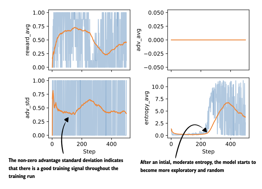Figure 7.9 Plots visualizing advantage statistics and entropy tracked during the GRPO training run (next to the average reward, which we tracked previously).

Let’s begin by analyzing the advantage shown in figure 7.9. As expected with GRPO-style normalization, the average advantage stays at zero throughout training. Since advantages are computed relative to the group mean, they sum to zero by design. As mentioned earlier, in practice, this metric mainly serves as a sanity check. If the advantage averages were to drift away from zero, that would point to a bug or a normalization issue.

The standard deviation of the advantages is more informative. Early in training, we see relatively high variance, which indicates that the model is producing rollouts with a wide range of quality. Over time, the advantage standard deviation gradually decreases and stabilizes, which means that the rollouts become more similar in quality. The key point is that as long as the advantage standard deviation remains nonzero and reasonably stable (meaning the value doesn’t vary much), there is still a usable learning signal and training happening.

Next, let’s look at the entropy. Early in training, the entropy is relatively low and fairly flat, which indicates that the model behaves in a largely deterministic way. In practice, increasing the sampling temperature would lead to more diverse rollouts, although it does not change the underlying entropy of the model itself.

Later in training, after roughly step 200, the entropy increases quite noticeably. This means that the next-token probabilities are more spread out and the model behaves more randomly. Very low entropy can also be a sign of collapse, where the model repeatedly produces the same or very similar outputs. In this run, considering the entropy together with the increasing average reward and the non-vanishing advantage standard deviation suggests still somewhat healthy exploration rather than collapse. This is also consistent with the earlier MATH-500 evaluation accuracy that stays in the 30%-40% range, which is not great but not near zero.

The main takeaway here is that each metric tells a slightly different part of the story, and they are most useful when considered together and in context.

7.4 Stabilizing sequence-level GRPO using clipped policy ratios

So far, we have mainly focused on analyzing the GRPO training results. Next, we start making additions to the GRPO algorithm itself. The version we have used so far is a simplified form of GRPO, and in this section we introduce a clipped policy ratio in the GRPO loss, as illustrated in the overview in figure 7.10.

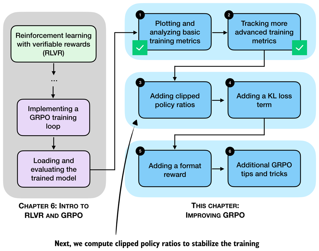Figure 7.10 After plotting basic and advanced GRPO training metrics, we now modify the GRPO algorithm and add clipped policy ratios.

The clipped policy ratios mentioned in figure 7.10 help limit overly large model weight updates and make training more stable, especially over longer runs. Ideally, we want to see that the model performance doesn’t noticeably decline as we have seen previously.

7.4.1 Computing clipped policy ratios

The clipped policy ratio measures how much the current policy, that is, the LLM being trained, has changed relative to an earlier version of itself. Concretely, it compares sequence logprobs computed before an update step with those computed after the update. You can think of it as asking: “If the LLM previously assigned a certain likelihood to this answer, how much more or less likely does it consider the same answer after we adjusted its weights?”

In the GRPO pipeline shown in figure 7.11, this corresponds to comparing the logprobs from step 4, which are computed using the old weight parameters, with the logprobs produced by the updated model (the model is updated via step 6).

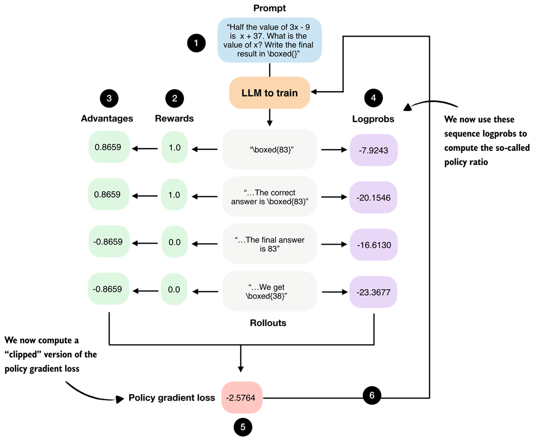Figure 7.11 GRPO overview figure from chapter 6. We now use the sequence logprobs from step 4 to compute policy ratios and clipped policy ratios.

Figure 7.11 shows the logprobs that are computed via the model that is being trained. The model is then updated via step 6. The policy ratios are computed from logprobs of the model in two different states: before and after a weight update. This will become clearer once we implement this concept in code. But first, to recap, in chapter 6 we computed the policy gradient loss as follows:

Listing 7.6 Compute policy gradient

# ...
 

rewards = torch.tensor([1., 1., 0., 0.]) # B
 

logprobs = torch.tensor([-7.9243, -20.1546, -16.6130, -23.3677]) # C
 
advantages = (rewards - rewards.mean()) / (rewards.std() + 1e-4)
 
pg_loss = -(advantages.detach() * logprobs).mean()
print("Policy gradient loss:", pg_loss)

• A: Code to compure rollouts omitted for brevity (not shown, implied)
• B: Compute rewards
• C: Compute sequence logprobs

The resulting policy gradient value, also as shown in figure 7.11, is -2.5764.

Next, we compute the policy ratio and clipped policy ratio, as shown in figure 7.12.

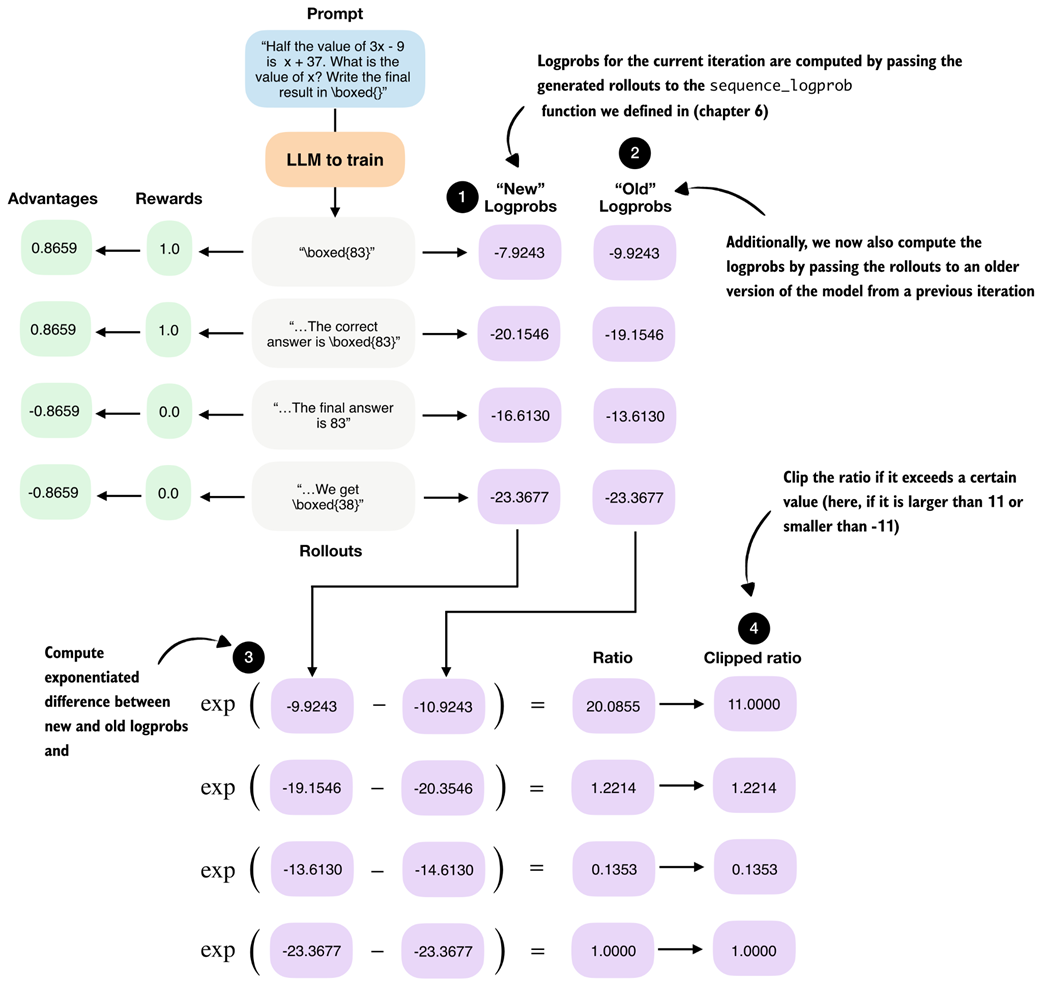Figure 7.12 Calculation of the policy ratio (ratio) and clipped policy ratio (clipped ratio) added to the GRPO from “new” and “old” logprobs.

The policy ratio and clipped policy ratio are computed by comparing log-probabilities from a previous version of the policy (“old” logprobs) with those from the current policy (“new” logprobs). The mathematical derivation is outside the scope of this chapter, but interested readers can find more details in the Proximal Policy Optimization Algorithms paper (https://arxiv.org/pdf/1707.06347).

For the following code-based illustration of the calculation shown in figure 7.12, we reuse the logprobs from the example above as old_logps, assume that a model update has taken place, and then compute the corresponding new_logps using the updated model. In practice, both would be computed using the same prompt to ensure a fair, apples-to-apples comparison between the old and current policy:

Listing 7.7 Compute policy ratios and clipped policy ratios:

new_logps = logprobs
 

old_logps = torch.tensor([
    -10.9243,   # -7.9243
    -20.3546,   # -20.1546
    -14.6130,   # -16.6130
    -23.3677,   # -23.3677
])
 
log_ratio = new_logps - old_logps
ratio = torch.exp(log_ratio)
clip_eps = 10.0
clipped_ratio = torch.clamp(ratio, 1.0 - clip_eps, 1.0 + clip_eps)
 
print("Ratio:        ", ratio)
print("Clipped ratio:", clipped_ratio)

• A: The values of the new_logps are shown side by side in the comments

The resulting unclipped and clipped policy ratios are shown below:

Ratio:         tensor([20.0855,  1.2214,  0.1353,  1.0000])
Clipped ratio: tensor([11.0000,  1.2214,  0.1353,  1.0000])

The ratio tells us how different the old and new logprobs are. If they are identical, the ratio is 1.0.

The clipped_ratio, which we use to compute a clipped version of the policy gradient loss, limits how far the new policy is allowed to move away from the old one in a single update. Concretely, if the new model suddenly assigns a much higher or much lower probability to a rollout compared to the old model, the raw ratio can become very large or very small. Without clipping, this would scale the advantage term substantially, which can lead to a very large gradient step that potentially destabilizes the training.

Using the clip_eps parameter in the previous code example, in practice, it is common to clamp the ratio to the range 1 ± clip_eps. For example, DeepSeek-R1 used clip_eps = 10, which corresponds to very weak clipping, while other RL training setups (for example, reinforcement learning with human feedback using the PPO algorithm) often use much smaller values such as 0.1.

As we can see, based on this very generous clip_eps value, only the first value is clipped from 20.0855 down to 11.0000.

Next, we apply the ratio and clipped_ratio in the loss computation. Previously, we multiplied the advantages directly by the logprobs. Now, we instead scale the advantages by the policy ratios and use the clipped objective to limit how much each rollout can influence the update:

Listing 7.8 Compute clipped policy gradient loss

adv = advantages.detach() # A
 
unclipped = ratio * adv
clipped = clipped_ratio * adv
 
obj = torch.where(
    adv >= 0, # B
    torch.minimum(unclipped, clipped), # C
    torch.maximum(unclipped, clipped), # D
)
 
clipped_pg_loss = -torch.mean(obj)
policy_ratio = torch.mean(ratio)
 
print("Clipped policy gradient loss:", clipped_pg_loss)
print("Policy ratio:", policy_ratio)

• A: Treat advantages as fixed learning signals (no backprop through rewards)
• B: Choose the more conservative update depending on the advantage signal
• C: Cap large positive updates
• D: Cap large negative updates

The resulting clipped policy gradient loss is -2.3998, which is slightly lower than the regular policy gradient loss we computed previously in this section (-2.5764). This small difference makes sense, because in our example, only one of the policy ratios was effectively clipped via the generous clip_eps=10.0 ratio. In general, this clipping can prevent overly aggressive updates that could destabilize training. Often, aggressive updates can move the policy too far in a single step, which can cause large shifts in token probabilities and then lead to reward crashes and entropy collapses, or other related problems.

In addition, we also compute the average policy ratio, policy_ratio = torch.mean(ratio), which we can track and report in the training run. Here, the result is a relatively large 5.6106. The large policy ratio in this example means that the updated policy (model) assigns a much higher probability to the sampled tokens than the previous policy.

7.4.2 Training with clipped policy ratios

We can apply the discussed clipped policy ratio and policy loss computations from listings 7.7 and 7.8 to see if they help stabilize the training.

The modified code can be downloaded from the supplementary materials as follows:

download_from_github(
    "ch07/03_rlvr_grpo_scripts_advanced/7_4_plus_clip_ratio.py"
)

And we can run it similar to before:

uv run 7_4_plus_clip_ratio.py \
    --steps 500  \
    --max_new_tokens 1024

As discussed in the previous section, the policy ratio compares logprobs computed under the current policy with those from a previous version of the policy.

DeepSeek-R1 generates a large pool of rollouts (8,192) and splits them into 16 minibatches to iterate over when updating the model using the clipped policy ratios:

1. Make a copy of the current model as the reference policy
2. Sample a big rollout pool using the reference policy
3. Split those fixed rollouts into minibatches
4. For each minibatch: a. Compute old_logps under the reference model b. Compute new_logps under the current model (which changes after each minibatch update) c. Update the current model
5. Update the reference model

Due to resource constraints, we can’t generate as many rollouts and minibatches as DeepSeek-R1 does and have to use workarounds. So, the procedure in the 7_4_plus_clip_ratio.py script is as follows:

1. Make a copy of the current model as the reference policy
2. Sample 8 rollouts using the reference policy
3. Then, we: a. Compute old_logps under the reference model b. Compute new_logps under the current model c. Update the current model
4. Repeat steps 2 and 3 (by default one more time) with different rollouts, instead of using minibatches
5. Update the reference model

In short, DeepSeek-R1 generates a huge rollout pool once, and then walks through it in minibatches. In our code, we generate a small batch of rollouts multiple times.

A log file of the 7_4_plus_clip_ratio.py script training run can be downloaded and visualized as follows:

download_from_github(
    "ch07/02_logs/7_4_plus_clip_ratio_metrics.csv"
)
plot_grpo_metrics(
    "7_4_plus_clip_ratio_metrics.csv",
    columns=["loss", "reward_avg", "avg_response_len", "eval_acc"]
)

Figure 7.13 shows the resulting plot.

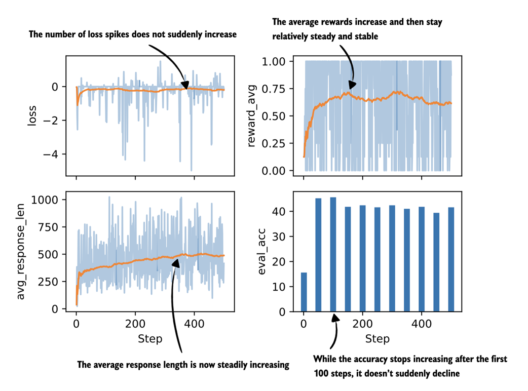Figure 7.13 Selected metrics from a GRPO training run using clipped policy ratios.

Compared to the previous training runs, the training with clipped policy ratios in figure 7.13 is indeed more stable as there is no visible drop in the average reward or evaluation accuracy around the 400-step mark. Optionally, we can also plot and inspect the other metrics, such as "policy_ratio", "adv_avg", "adv_std", "entropy_avg", which is left as an exercise for the reader.

7.5 Controlling how much the model changes with a KL term

Previously, we skipped the KL loss term of the GRPO algorithm to keep the presentation manageable. To complete the GRPO algorithm, we now add the KL loss term as shown in figure 7.14.

Note

Readers familiar with reinforcement learning may recognize that what we implemented up to this point is essentially REINFORCE with group-normalized advantages.

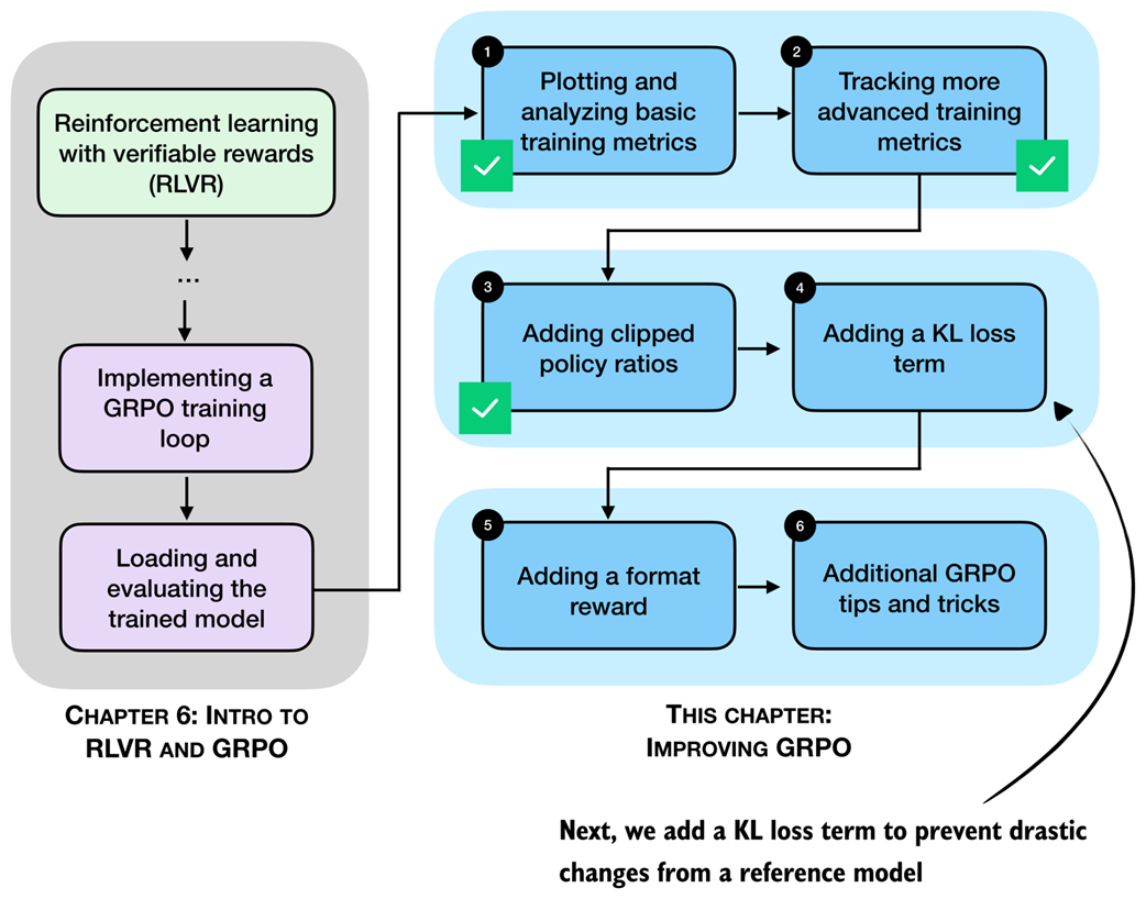Figure 7.14 In this section, we implement a KL loss term, which is a part of the original GRPO algorithm.

KL is short for Kullback-Leibler divergence and measures how much the current policy, that is, the LLM being trained, deviates from a reference policy, typically the original model at the start of training.

The KL term acts as a constraint (technically called a regularizer) that discourages overly large updates and keeps the model close to its original behavior to prevent drastic or unstable changes. This is closely related to the clipped policy ratios we introduced earlier. Using clipped policy ratios, we limited how large individual update steps can be. The KL term is another mechanism to control how much the model can change more long term over the training trajectory. While the clipped policy ratios are more focused on limiting the changes between each step, the KL term is often used to control the changes more long term over the training trajectory.

7.5.1 Implementing the KL loss term

Similar to when we computed the clipped policy ratio, calculating the KL term involves two sets of logprobs we compare, as shown in figure 7.15.

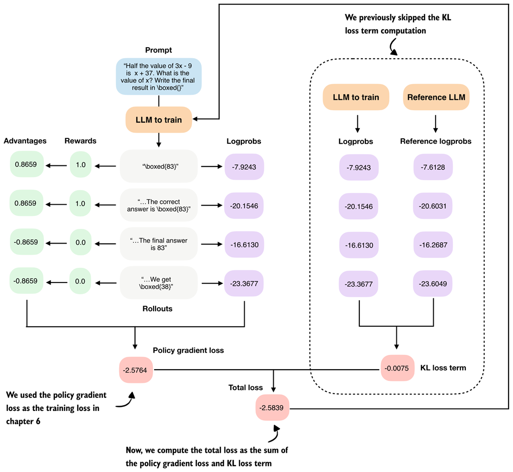Figure 7.15 Overview of the GRPO algorithm with the KL loss term calculation added to the right.

Figure 7.15 shows the KL loss term computation as part of the GRPO algorithm. The KL loss term calculations involve a comparison between logprobs and reference logprobs. It is computed by summing the differences between these corresponding logprobs. A small KL loss term value indicates that the current model and the reference model output relatively similar logprobs, meaning the current model has not changed much compared to the reference model. This is generally desirable for stability, as it prevents large, abrupt shifts in behavior. However, if the KL term remains too small for too long, it may also indicate that the learning rate is limited.

The resulting KL loss term is then added to the policy gradient loss to compute the total loss, so weight updates that strongly increase the difference (divergence) from the reference model (even if they result in a high reward) are penalized during training.

In the clipped policy ratio section, we replaced the reference model in each iteration. For the KL loss term, the reference model, which is used to compute the reference logprobs, is the original model at the beginning of the training and is either kept fixed or replaced relatively rarely (in the case of DeepSeek-R1, every 400 steps).

The following code illustrates how the compute_grpo_loss function can be modified to include this KL loss term. To avoid code duplication, the code in listing 7.9 does not show the fully modified compute_grpo_loss_with_kl, which focuses only on the changes we have to make to the compute_grpo_loss function.

The new additions are marked with comments or are located inside the if kl_coeff blocks.

Listing 7.9 Adding a KL term to the GRPO loss computation

import copy
 
kl_coeff = 0.0 # A
 
if kl_coeff:
    ref_model = copy.deepcopy(model).to(device)
    ref_model.eval()
    for p in ref_model.parameters():
        p.requires_grad = False # B
else:
    ref_model = None
 
 
def compute_grpo_loss_with_kl(
    model,
    ref_model, # C
    # ...
    kl_coeff=0.02, # D
):
    roll_logps, roll_ref_logps, roll_rewards, samples = [], [], [], []
    # ...
 
    for _ in range(num_rollouts):
        token_ids, prompt_len, text = sample_response(
        # ...
        )
 
        
        if kl_coeff:
            with torch.no_grad():
                ref_logp = sequence_logprob(
                    ref_model, token_ids, prompt_len
                ) # E
        else:
            ref_logp = None
 
        reward = reward_rlvr(text, example["answer"])
 
        roll_rewards.append(reward)
        roll_logps.append(logp)
        if kl_coeff:
            roll_ref_logps.append(ref_logp)
        
        # ...
 
    rewards = torch.tensor(roll_rewards, device=device)
    advantages = (rewards - rewards.mean()) / (rewards.std() + 1e-4)
 
    logps = torch.stack(roll_logps)
    if kl_coeff:
        ref_logps = torch.stack(roll_ref_logps).detach()
 
    pg_loss = -(advantages.detach() * logps).mean()
 
    
    if kl_coeff:
        kl_loss = kl_coeff * torch.mean(logps - ref_logps) # F
    else:
        kl_loss = torch.tensor(0.0, device=logps.device)
 
    
    loss = pg_loss + kl_loss # G

• A: kl_coeff = 0.0 deactivates the KL term and the code is similar to before
• B: Make copy of the original model and disable gradients so it isn’t updated
• C: New: Pass reference model
• D: New: Specify KL strength
• E: Compute logprobs with reference model
• F: Compute KL loss term
• G: New: Add KL loss term to policy gradient loss

Note that adding the KL loss term increases resource usage, since we now need to keep an additional copy of the original model. The strength of this penalty is controlled by kl_coeff. Larger kl_coeff values add a stronger constraint on how far the current policy is allowed to change from the reference model.

The setting kl_coeff = 0.0 at the top of listing 7.9 is only added so that if we were to run this abbreviated code snippet in a code environment, it wouldn’t crash. In practice, kl_coeff is typically a small value between 0.001 and 0.05.

7.5.2 Training with a KL loss term

The following script from the supplementary materials implements the KL loss term code modification we discussed previously:

download_from_github(
    "ch07/03_rlvr_grpo_scripts_advanced/7_5_plus_kl.py"
)

Similar to before, we can run it as follows:

uv run 7_5_plus_kl.py \
    --steps 500  \
    --max_new_tokens 1024

Let’s take a look at the log files from a training run that was executed with the settings shown above:

download_from_github(
    "ch07/02_logs/"
    "7_5_plus_kl_metrics.csv"
)
plot_grpo_metrics(
    "7_5_plus_kl_metrics.csv",
    columns=["loss", "reward_avg", "avg_response_len", "eval_acc"]
)

The resulting plots are shown in figure 7.16.

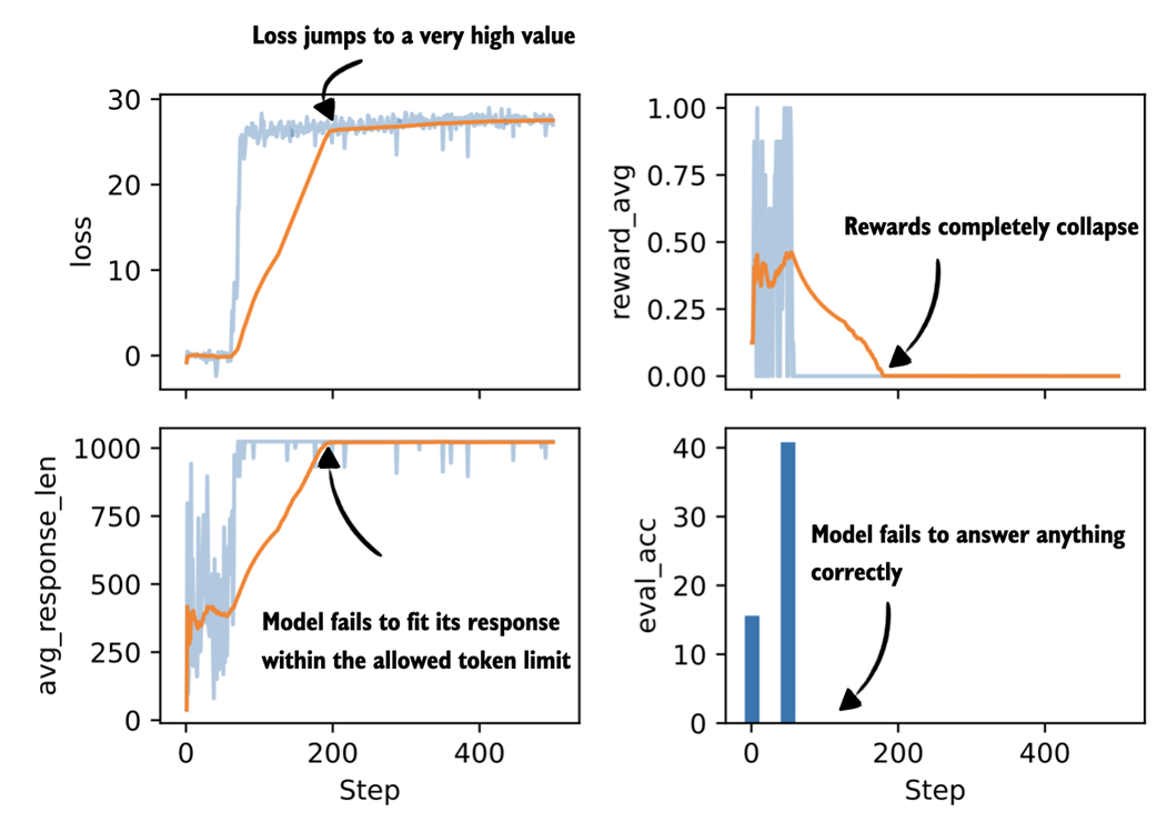Figure 7.16 Selected metrics from a GRPO training run after adding a KL loss term.

We can see that the first fifty steps improve the model performance noticeably from slightly above 15% accuracy to approximately 40% accuracy. We then see a total collapse where the loss values explode and the average reward goes towards 0. This is accompanied by a crash in the evaluation accuracy that also goes towards 0%.

On manual inspection of generated responses, the model eventually started producing nonsensical text and random tokens, such as framework.raises Self profess(import. There are a couple of likely reasons for this behavior.

First, the KL term is computed using summed logprobs over the answer tokens, that is, kl_loss = kl_coeff * mean(new_logps - ref_logps). As a result, longer sequences naturally lead to larger KL values. This can unintentionally encourage very long outputs, which we also observe in the growing response length, and can destabilize training.

Second, once rewards collapse to 0 around step 200, the KL term becomes the only remaining source of gradient signal. When all rewards are zero, the advantages are zero as well, so the policy gradient loss no longer contributes any gradient. The KL term is still active and starts to dominate the updates. This means the KL loss term can push the model toward higher entropy and near-uniform token distributions, which explains both the increasingly random outputs and the drop to 0.0% evaluation accuracy. If you want, you can plot the other evaluation metrics, for instance, "policy_ratio", "adv_avg", "adv_std", "entropy_avg", and confirm that the entropy becomes very large.

While the KL term is a standard part of the GRPO algorithm, which is why we introduce it here, several recent works report that models can train better without it. Examples include Dr. GRPO, Llama 3, and DeepSeek-V3.2, all of which observe improved stability or performance when the KL term is reduced or omitted (see appendix C for more detailed references).

Improving Training Stability with a KL Term

Alternatively, instead of removing the KL term, there are several ways to improve training stability. First, we can reduce kl_coeff from 0.02 to a smaller value (for example, 0.001) to weaken the KL penalty, although in my experiments this was not sufficient.

Since we saw that response length keeps growing until it hits the maximum, another option is to length-normalize the sequence logprobs by dividing by the number of generated tokens, which approximates average per-token logprobs. This could reduce the incentive to increase response length to accumulate larger absolute logprob differences.

A third option is to use a reweighted KL term based on importance sampling, as proposed by DeepSeek-V3.2. Instead of

kl_loss = kl_coeff * torch.mean(logps - ref_logps)
# we use
kl_loss = (
    kl_coeff * torch.mean(torch.exp(new_logps - old_logps)
    * (new_logps - ref_logps)
)

Here, the importance weight torch.exp(new_logps - old_logps) corrects for rollouts being generated by the old policy, and it downweights samples that the current policy would rarely produce and upweights those it would.

Finally, we could add a small format reward to prevent advantages from collapsing to zero (we will revisit format rewards in the next section).

That said, for math data, a common recommendation is to omit the KL term altogether (e.g., Dr. GRPO, Llama 3, and DeepSeek-V3.2), which also simplifies the code and reduces resource requirements since we don’t have to keep an additional reference model in memory.

7.6 Adding an explicit format reward

So far, we only used one type of verifiable reward, an answer-correctness reward, when training the model. In practice, this is sufficient to train reasoning models with RLVR. It is also common to use one or more auxiliary rewards, for example, a format reward that checks whether the generated answer follows certain formatting guidelines (figure 7.17).

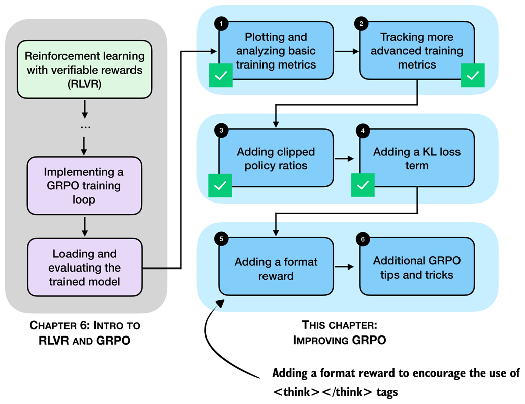Figure 7.17 In this section, we implement a format reward that encourages the model to generate <think>...</think> tokens

Specifically, we will focus on a format reward that encourages the model to use so-called <think>...</think> tokens, as shown in figure 7.17.

7.6.1 Using <think> tokens

Some reasoning models, such as DeepSeek-R1 and Qwen3, use special <think> and </think> tokens. These <think> tokens are ordinary text tokens that mark the beginning and end of the model’s intermediate reasoning. In practice, we can prompt the model to write its step-by-step reasoning inside <think> ... </think> and then provide the final answer outside these tags. This entire approach is optional, but it makes the output structure explicit and helps separate reasoning from the final result.

To start illustrating this concept, we load the tokenizer of the base model we used earlier.

Listing 7.10 Loading the base model tokenizer

from reasoning_from_scratch.ch02 import get_device
from reasoning_from_scratch.ch03 import load_model_and_tokenizer
 
device = get_device()
model, tokenizer_base = load_model_and_tokenizer(
    which_model="base",
    device=device,
    use_compile=False
)

Next, let’s use the tokenizer to encode <think>:

print(tokenizer_base.encode("<think>"))

The output is [13708, 766, 29], which means that the tokenizer breaks up the <think> token into several subword tokens, which indicates that the <think> token is not part of the tokenizer’s vocabulary.

Nowadays, when developing tokenizers and creating the embedding layers of LLMs, the developers often leave some unused placeholder token IDs that can be used for specific purposes when fine-tuning a model. In this case, the Qwen3 base model tokenizer has some empty placeholder slots that we can use to add the <think>:

tokenizer_base._tok.add_special_tokens(
  ["<tool_response>", "</tool_response>", "<think>", "</think>"]
)

Note that we also added the <tool_response> and </tool_response> tokens above to match it up with the tokenizer of the Qwen3 reasoning variant, which we will discuss shortly. But first, let’s check if the modified base tokenizer now supports the newly added <think> and </think> tokens:

print(tokenizer_base.encode("<think>"))
print(tokenizer_base.encode("</think>"))

The outputs are single tokens [151667] and [151668], which indicate that the <think> and </think> tokens are now part of the vocabulary and are no longer broken up into subword tokens.

These new tokens would also be supported by the base model, which supports token IDs from 0 to 151935 as it has a vocabulary size of 151936, which we can confirm by printing the size of the embedding layer:

print("Vocabulary size:", model.tok_emb.weight.shape[0])

Alternatively, instead of modifying the base tokenizer, the tokenizer of the reasoning model variant already supports these <think> tokens natively, which means that we don’t have to modify the tokenizer manually. For instance, similar to what we have done in chapter 2, we can load the tokenizer separately:

Listing 7.11 Loading the reasoning model tokenizer

from reasoning_from_scratch.qwen3 import Qwen3Tokenizer
from reasoning_from_scratch.qwen3 import download_qwen3_small
 
download_qwen3_small(
    kind="reasoning", tokenizer_only=True, out_dir="qwen3"
)
 
tokenizer_path = Path("qwen3") / "tokenizer-reasoning.json"
tokenizer = Qwen3Tokenizer(tokenizer_file_path=tokenizer_path)

Now, let’s use the reasoning tokenizer (tokenizer) instead of the tokenizer_base to encode the token IDs similar to what we have done earlier:

print(tokenizer.encode("<think>"))
print(tokenizer.encode("</think>"))

Similar to when we used tokenizer_base, this returns [151667] and [151668].

Now that we have a tokenizer that supports these <think> &lt;/think> tokens, we can then develop a reward function that checks whether the LLM uses these tokens and provides a non-zero reward if it does, as illustrated in figure 7.18.

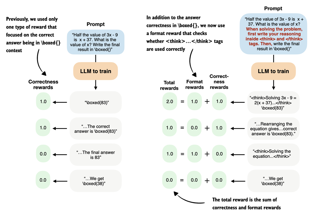Figure 7.18 Illustration of using the previous correctness reward (left) and a correctness plus format reward (right).

Similar to figure 7.18, we develop a function that returns 1.0 if both <think> and </think> occur in the output and in the right order; otherwise, it returns 0.0:

Listing 7.12 Implementing a format reward function

def reward_format(
    token_ids,
    prompt_len,
    start_think_id=151667,
    end_think_id=151668,
):
    try:
        gen = token_ids[prompt_len:].tolist()
        return float(
            gen.index(start_think_id) < gen.index(end_think_id)
        )
    except ValueError:
        return 0.0

Let’s give this a try on a simple sample text:

prompt = "Calculate ..."
rollout = "Let's ... <think> ... </think> ..."
token_ids = tokenizer.encode(prompt + rollout)
reward_format(
    token_ids=torch.tensor(token_ids),
    prompt_len=len(tokenizer.encode(prompt))
)

Running the following code returns 1.0 as expected, since the answer (rollout) contains both <think> and </think>.

Exercise 7.1: Testing the <think> format reward

Run the example and confirm it returns 1.0, since both <think> and </think> appear in the correct order.

Now modify the rollout text by:

• Introducing a typo in one of the <think> </think> tags
• Reversing the tag order
• Removing one tag

Verify that the reward becomes 0.0 in each case.

Using this new reward_format function, we can use the format reward as an additional reward signal to train the model. For instance, we could convert the compute_grpo_loss from chapter 6 into a compute_grpo_loss_plus_format_reward function as follows (the changes are highlighted in the comments):

Listing 7.13 Updating the GRPO loss function with a format reward

def compute_grpo_loss_plus_format_reward(
    # ...
    format_reward_weight=1.0, # A
):
    # ...
 
        logp = sequence_logprob(model, token_ids, prompt_len)
        rlvr_reward = reward_rlvr(text, example["answer"])
 

        format_reward = reward_format(token_ids, prompt_len)         # NEW B
        reward = rlvr_reward + format_reward_weight * format_reward  # NEW
 
    # ...

• A: A setting parameter that lets us regulate the magnitude of the format reward relative to the existing correctness reward
• B: New format reward lines that modify the previous reward to now consist of a correctness and a format reward

In addition, we can modify the render_prompt to direct the model to emit these <think> and </think> tokens explicitly:

Listing 7.14 Updated prompt rendering function for <think> tokens

def render_prompt_with_think_tokens(prompt):
    template = (
        "You are a helpful math assistant.\n"
        "When solving the problem, first write your reasoning inside <think> and </think> tags.\n"
        "Then write the final result on a new line in the exact format:\n"
        "\\boxed{ANSWER}\n\n"
        f"Question:\n{prompt}\n\nAnswer:"
    )
    return template

In theory, the modifications in the previous code listings 7.11 to 7.14 should be sufficient to train a reasoning model with an additional format reward. The next section will explain how this works in practice and discuss additional caveats.

7.6.2 Training a model to emit <think> tokens

Similar to previous sections, the modifications needed to train a reasoning model including a formatting reward are implemented in a script that we can download from the supplementary materials:

download_from_github(
    "ch07/03_rlvr_grpo_scripts_advanced/7_6_plus_format_reward.py"
)

There are a few caveats about this script to keep in mind. For instance, if we train the base model with the modified prompt to emit <think> and </think> tokens, as shown in listing 7.14, the results would be quite poor because the base model has never seen these tokens before.

Instead, the proper way to introduce these new tokens would be to pre-train or instruction fine-tune the model on data that includes <think> and </think> tokens first (instruction fine-tuning is covered in the next chapter).

So, for this chapter, where we focus on reinforcement learning, we train the existing 'reasoning' variant of the model, which is already familiar with <think> tokens. (This is the same 'reasoning' variant we introduced in chapter 3).

Similar to before, we can run the script as follows:

uv run 7_6_plus_format_reward.py \
    --steps 500  \
    --max_new_tokens 1024

Note that this script is already configured to use the 'reasoning' model variant instead of the 'base' model.

Also, similar to before, we can download a log file of this run for further analysis, as running the experiment can be resource-intensive and expensive:

download_from_github(
    "ch07/02_logs/7_6_plus_format_reward_metrics.csv"
)
plot_grpo_metrics(
    "7_6_plus_format_reward_metrics.csv",
    columns=["loss", "reward_avg", "avg_response_len", "eval_acc"]
)

The resulting plot is shown in figure 7.19.

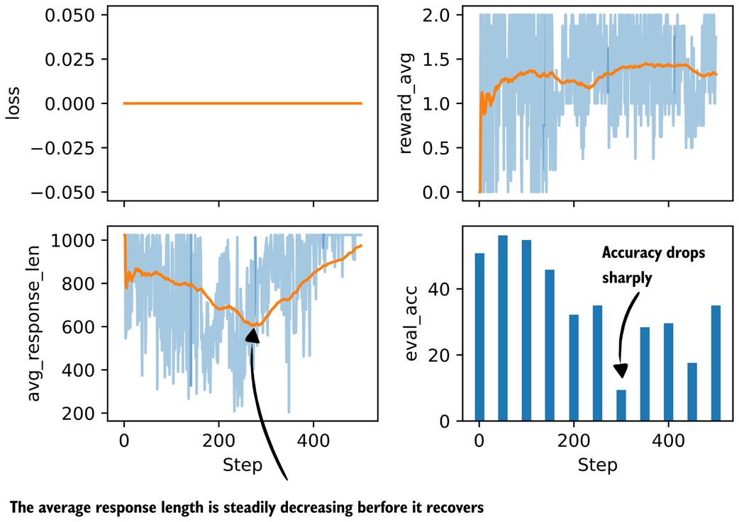Figure 7.19 Basic metrics from a GRPO training run with a format reward.

As we can see in figure 7.19, the model improves at first but then starts to get worse in terms of evaluation accuracy while the average reward stays approximately constant. The decline in evaluation accuracy appears to correlate with the shorter response lengths the model produces after that point.

To investigate this further, let’s also have a look at some additional metrics:

plot_grpo_metrics(
    "7_6_plus_format_reward_metrics.csv",
    columns=["reward_avg", "format_reward_avg", "adv_std", "entropy_avg"],
)

The results are shown in figure 7.20.

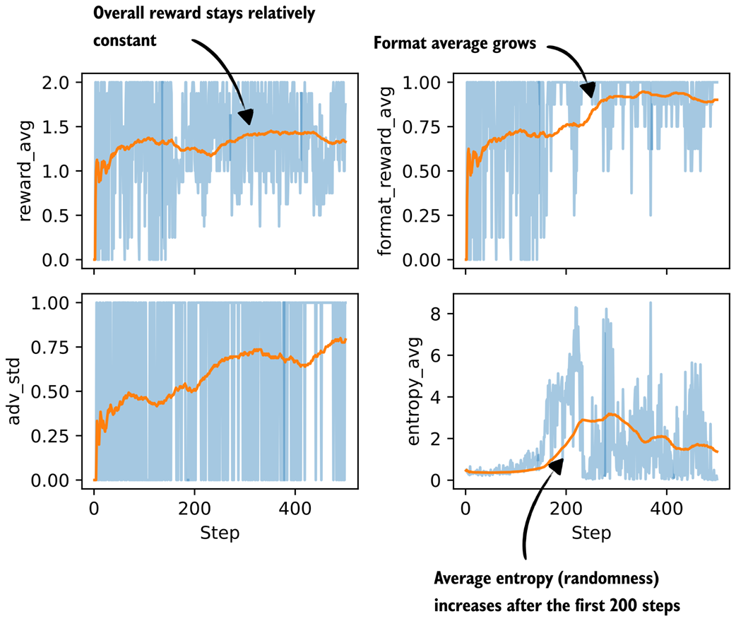Figure 7.20 Additional metrics from a GRPO training run with a format reward.

As figure 7.20 shows, one possible explanation for the declining model performance is that the model receives too much reward from simply following the <think> tag format, as shown in the format_reward_avg plot in figure 7.20. In other words, the model does not focus enough on answer correctness (see reward_avg).

One way to potentially address this is to reduce the strength of the format reward, for example by lowering the default format_reward_weight from 1.0 to 0.1. Another option is to make the format reward conditional, so that it is only applied when the answer is also correct. In the current setup, the format reward is granted regardless of correctness.

Exercise 7.2: Making the format reward conditional

Modify the format reward calculation

reward = rlvr_reward + format_reward_weight * format_reward

so that the format reward is only given if the correctness reward (rlvr_reward) is non-zero. Repeat the training run with the conditional format reward. Does conditioning the format reward change training behavior and final accuracy?

Note: Since running these experiments can be resource-intensive, reference results are provided in appendix C.

7.6.3 More GRPO modifications, tips, and tricks

Previously, we implemented a version of GRPO without KL loss term and clipped policy ratios, and format reward for introductory purposes. Then, we added these additional concepts to get a solid foundation and understanding of the original GRPO algorithm, which underlies most of the modern reasoning training frameworks. Figure 7.21 briefly shows this next step which is additional modifications, tips, and tricks.

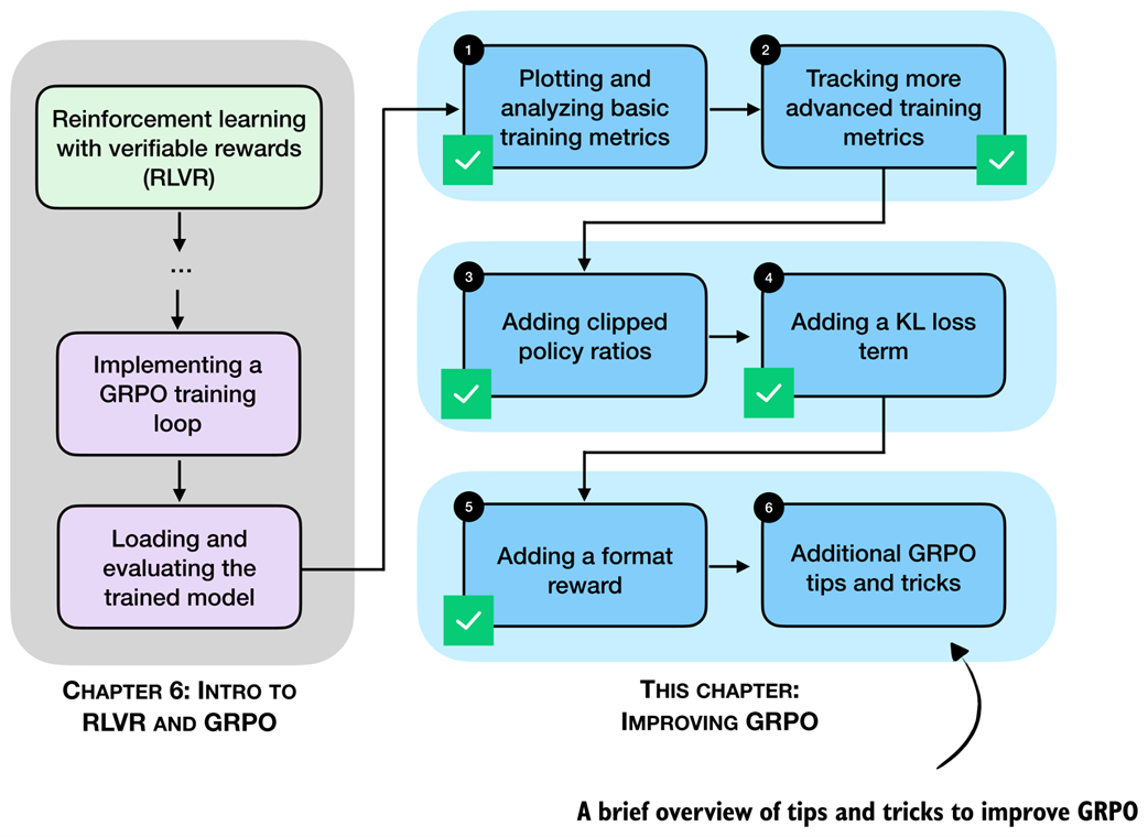Figure 7.21 This last section in this chapter outlines some additional GRPO modifications that emerged in recent months.

As far as RLVR with GRPO goes, we learned that there are many knobs to tune. Besides changing the basic settings such as the learning rate, maximum response length, prompt format, and so on, there is a near infinite number of settings and modifications to try, where exploring a single modification or a small handful of modifications thoroughly can be a whole month- or year-long research project for a small research team.

It is expected that algorithms keep changing and evolving. It is important, though, to understand the fundamentals and general idea behind it to also understand and appreciate these improvements.

In the months following the success of DeepSeek-R1, many researchers proposed changes to the original GRPO algorithm that improved both training stability and final performance. To provide a taste of several suggested improvements, below is a selection from RLOO, Dr. GRPO, DeepSeek-V3.2, and others (you can find a full list of references and links in appendix C):

1. Poor gradient signal filtering (GRPO)
2. Active sampling (GRPO)
3. Switch from sequence- to token-level loss (RLOO)
4. No KL loss (GRPO and Dr. GRPO)
5. Clip higher (GRPO)
6. Truncated importance sampling (PPO2)
7. No standard deviation normalization (Dr. GRPO)
8. KL tuning with domain-specific KL strengths; zero for math (DeepSeek-V3.2)
9. Reweighted KL (DeepSeek-V3.2)
10. Off-policy sequence masking (DeepSeek-V3.2)
11. Keep sampling mask for top-k / top-p (DeepSeek-V3.2)
12. Keep original GRPO advantage normalization (DeepSeek-V3.2)
13. Pre-reward group-wise normalization before aggregating (GRPO)
14. Sequence-level importance sampling and clipping (GRPO)
15. Clip importance-sampling weights rather than token updates (PPO2)

Given the already substantial length here, detailed explanations, code examples, and training run results concerning those modifications are outside the scope of this chapter. If you’re interested, you can find these in the supplementary materials at https://github.com/rasbt/reasoning-from-scratch/tree/main/ch07/03_rlvr_grpo_scripts_advanced.

7.7 Summary

• Training reasoning models with GRPO can become unstable over longer runs, even when the implementation is correct and rewards initially improve.
• Interpreting GRPO training requires tracking multiple metrics jointly (average rewards, response length, evaluation accuracy, advantage statistics, and entropy)
  • Basic metrics such as loss mainly serve as sanity checks in GRPO and should not be over-interpreted in isolation.
  • Advantage statistics provide useful diagnostics: the mean should remain near zero by design, while the standard deviation reflects the strength and stability of the learning signal.
  • Entropy measures how uncertain the model is during generation. Very low entropy can signal collapse, and very large entropy can indicate unstable updates and randomness in the model responses.
• Clipped policy ratios limit how much the policy can change between updates and can substantially improve training stability over longer runs.
• Adding a KL divergence term constrains long-term drift from a reference model but can destabilize training when rewards collapse.
• For math reasoning tasks, several recent systems report better stability and performance by omitting the KL term altogether.
• Auxiliary format rewards can improve the response structure, such as encouraging the use of <think> and </think> tokens.
• Beyond the original GRPO algorithm, many recent extensions modify advantage normalization, importance sampling, clipping strategies, and KL handling to improve stability and efficiency.