Qwen3 LLM source code
Appendix C. Qwen3 LLM source code
While this is a from scratch book, as mentioned in the main chapters, the from scratch part refers to the reasoning techniques, not the LLM itself. Implementing an LLM entirely from scratch would require a separate book, which is the topic of my Build A Large Language Model (From Scratch) book (http://mng.bz/orYv).
However, for readers interested in seeing the Qwen3 implementation we use in this Build A Reasoning Model (From Scratch) book, this appendix lists the source code for the Qwen3Model model that I implemented in and that we import from the book’s reasoning_from_scratch Python package:
from reasoning_from_scratch.qwen3 import Qwen3Model, Qwen3Tokenizer
As shown in figure C.1, the Qwen3 architecture is very similar to GPT-2, which is covered in my Build A Large Language Model (From Scratch) book. While familiarity with GPT-2 is not required for this book, this appendix mentions comparisons to GPT-2 for those who are familiar with it. In fact, I wrote the Qwen3 implementation by porting the GPT-2 model from my other book piece by piece into the Qwen3 architecture, such that it follows similar style conventions to improve readability.
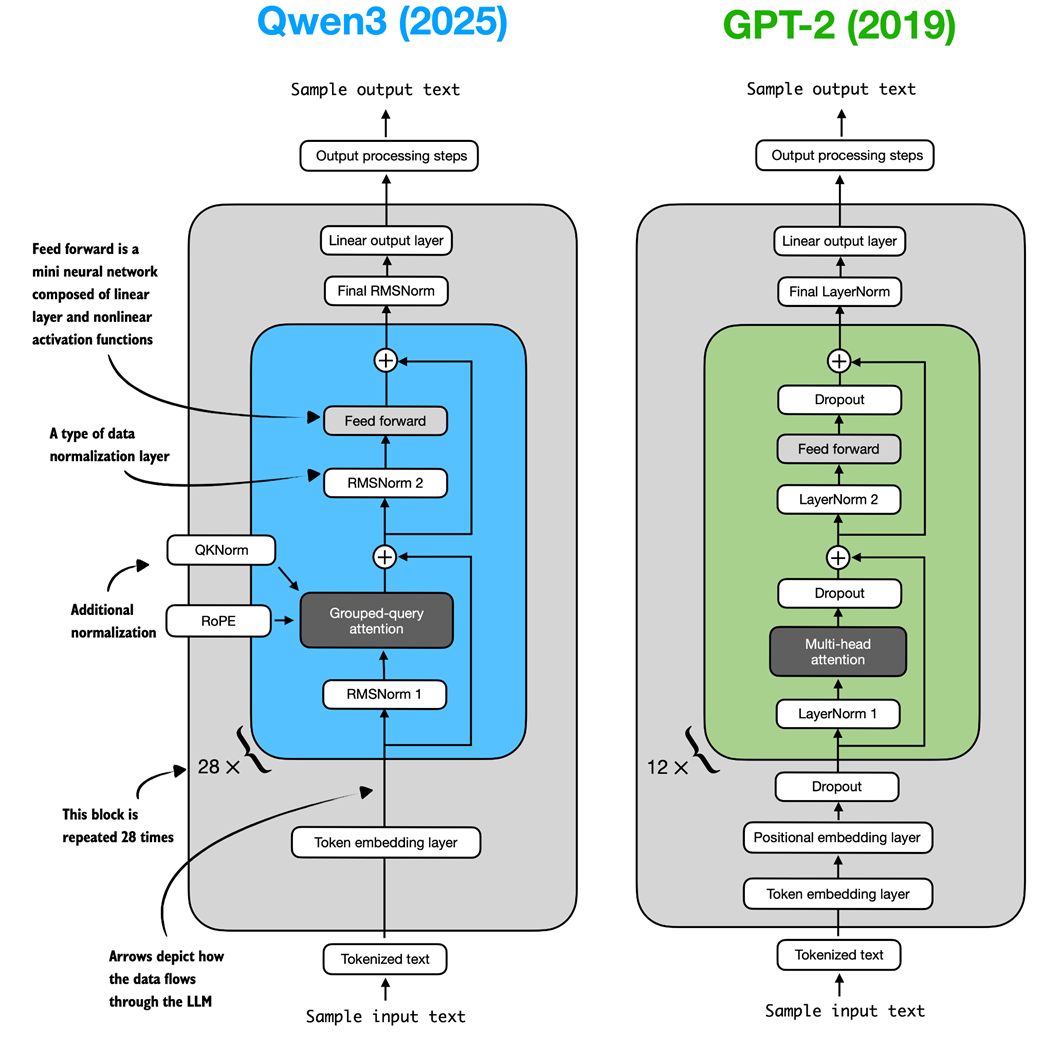 Figure C.1 Architectural comparison between Qwen3 and GPT-2. Both models process text through embedding layers and stacked transformer blocks, but they differ in certain design choices.
As shown in figure C.1, both Qwen3 (released in 2025) and GPT-2 (released in 2019) are very similar overall in that they are both based on the decoder modules of the original transformer architecture. However, some of the design choices have evolved since 2019. Note that most of these design choices found in Qwen3 are not unique to Qwen3 but are found in many other contemporary LLMs, which I discussed in my The Big LLM Architecture Comparison (https://magazine.sebastianraschka.com/p/the-big-llm-architecture-comparison) article.
For readers new to LLMs who want to understand how these architectures are implemented, I recommend starting with GPT-2. Its design is simpler to implement, which makes it an easier entry point before exploring more modern variations.
Since this book does not focus on architecture implementations, the remainder of this appendix will cover only a brief overview of Qwen3’s code.
C.1 Root mean square layer normalization (RMSNorm)
In contrast to GPT-2, which used standard LayerNorm, the newer Qwen3 architecture replaces it with root mean square layer normalization (RMSNorm). This is a trend that has become increasingly common in recent model architectures.
RMSNorm fulfills the same core function as LayerNorm: normalizing layer activations to stabilize and improve training. However, it simplifies the computation by removing the mean-centering step, as shown in figure C.2. This means that activations will still be normalized, but they are not centered at 0.
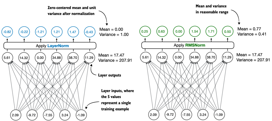 Figure C.2 Comparison of LayerNorm and RMSNorm. LayerNorm (left) normalizes activations so that their average value (mean) is exactly zero and their spread (variance) is exactly one. RMSNorm (right) instead scales activations based on their root mean square, which does not enforce zero mean or unit variance, but still keeps the mean and variance within a reasonable range for stable training.
As we can see in figure C.2, both LayerNorm and RMSNorm scale the layer outputs to be in a reasonable range.
LayerNorm subtracts the mean and divides by the standard deviation such that the layer outputs have a zero mean and unit variance (variance of one and standard deviation of one), which results in favorable properties, in terms of gradient values, for stable training.
RMSNorm divides the inputs by the root mean square. This scales activations to a comparable magnitude without enforcing zero mean or unit variance. In this particular example shown in figure C.2, the mean is 0.77 and the variance is 0.41.
Both LayerNorm and RMSNorm stabilize activation scales and improve optimization; however, RMSNorm is often preferred in large-scale LLMs because it is computationally cheaper. Unlike LayerNorm, RMSNorm does not use a bias (shift) term by default, which reduces the number of trainable parameters. Moreover, RMSNorm reduces the expensive mean and variance computations to a single root-mean-square operation. This reduces the number of cross-feature reductions from two to one, which lowers communication overhead on GPUs and slightly improves training efficiency.
Listing C.1 shows what RMSNorm looks like in code.
Listing C.1 RMSNorm
import torch.nn as nn

class RMSNorm(nn.Module):

    def __init__(
        self,
        emb_dim,
        eps=1e-6,
        bias=False,
        qwen3_compatible=True,
    ):
        super().__init__()
        self.eps = eps
        self.qwen3_compatible = qwen3_compatible
        self.scale = nn.Parameter(torch.ones(emb_dim))
        self.shift = nn.Parameter(torch.zeros(emb_dim)) if bias else None

    def forward(self, x):
        input_dtype = x.dtype

        if self.qwen3_compatible:
            x = x.to(torch.float32)

        variance = x.pow(2).mean(dim=-1, keepdim=True)
        norm_x = x * torch.rsqrt(variance + self.eps)
        norm_x = norm_x * self.scale

        if self.shift is not None:
            norm_x = norm_x + self.shift

        return norm_x.to(input_dtype)
Note that, for brevity, this appendix does not provide detailed code standalone for each LLM component. Instead, in section C.6, we will integrate all components into the Qwen3Model class, load the pre-trained weights into it, and then use this model to generate text in section C.9.
C.2 Feed forward module
The feed forward module (a small multi-layer perceptron) is replaced with a gated linear unit (GLU) variant, introduced in a 2020 paper (https://arxiv.org/abs/2002.05202). In this design, the standard two fully connected layers are replaced by three, as shown in figure C.3.
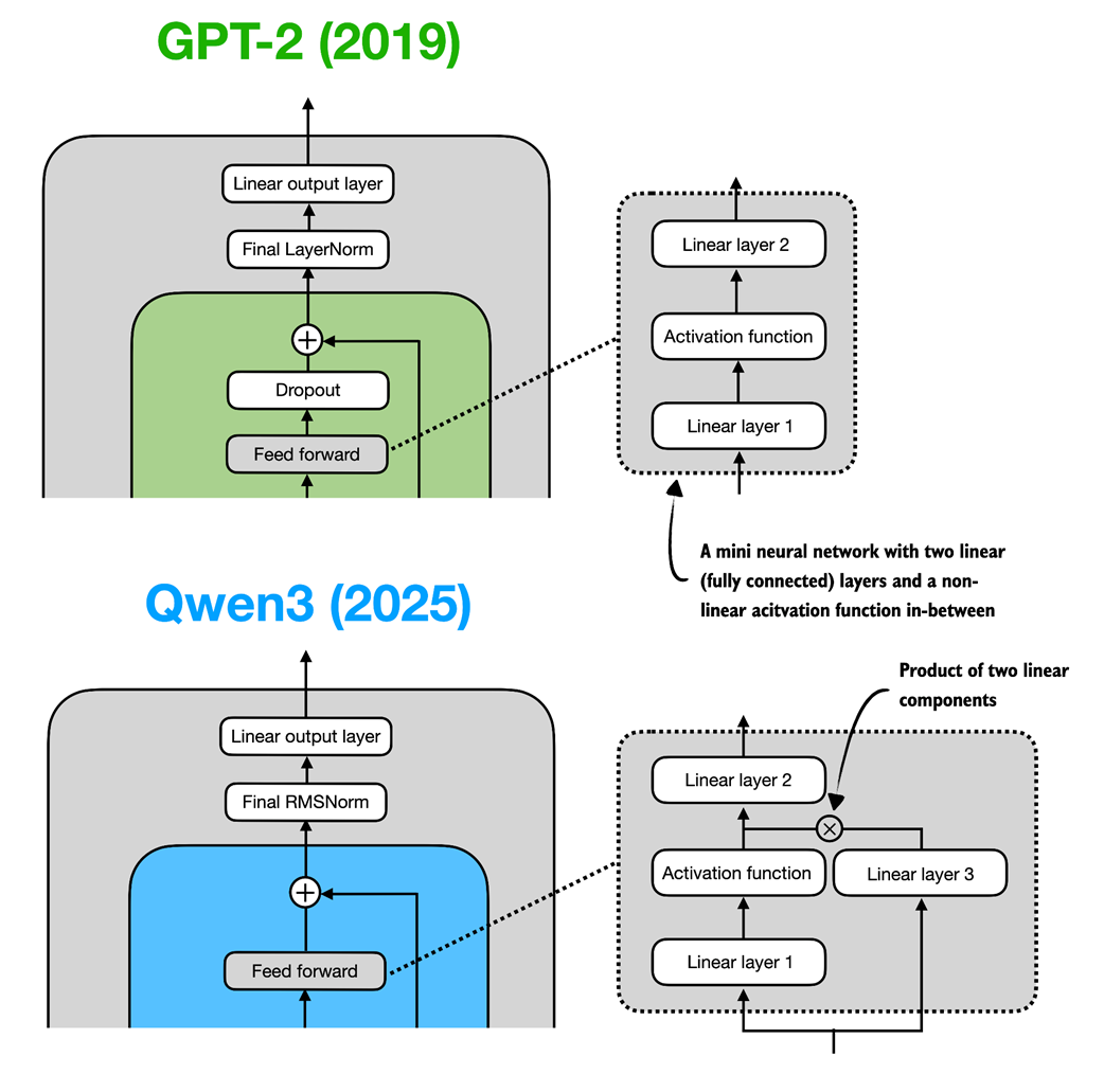 Figure C.3 In GPT-2 (top), the feed forward module consists of two fully connected (linear) layers separated by a non-linear activation function. In Qwen3 (bottom), this module is a gated linear unit (GLU) variant, which adds a third linear layer (linear layer 3) and multiplies the output of this linear layer 3 elementwise with the activated output of linear layer 1.
Qwen3’s feed forward module (figure C.3) can be implemented as shown in listing C.2.
Listing C.2 Qwen3 feed forward module
class FeedForward(nn.Module):
    def __init__(self, cfg):
        super().__init__()
        self.fc1 = nn.Linear(
            cfg["emb_dim"], cfg["hidden_dim"], dtype=cfg["dtype"],
            bias=False
        )
        self.fc2 = nn.Linear(
            cfg["emb_dim"], cfg["hidden_dim"], dtype=cfg["dtype"],
            bias=False
        )
        self.fc3 = nn.Linear(
            cfg["hidden_dim"], cfg["emb_dim"], dtype=cfg["dtype"],
            bias=False
        )

    def forward(self, x):
        x_fc1 = self.fc1(x)
        x_fc2 = self.fc2(x)
        # The non-linear activation function here is a SiLU function
        x = nn.functional.silu(x_fc1) * x_fc2
        return self.fc3(x)
At first glance, it might seem that the GLU feed forward variant used in Qwen3 should outperform the standard feed forward variant in GPT-2, simply because it adds an extra linear layer (three instead of two) and therefore appears to have more parameters.
However, this intuition is misleading. In practice, the fc1 and fc2 layers in the GLU variant are each half the width of the fc1 layer in a standard feed forward module. In practice, the GLU variant has fewer parameters.
To illustrate this with a concrete example, suppose the input dimension to the “Linear layer 1” in figure C.3 is 1024. This corresponds to cfg["emb_dim"] in listing C.2. The output dimension of fc1 is 3,072 (cfg["hidden_dim"]). Note that these are the actual numbers used in the Qwen3 0.6B variant. In this case, we have the following parameter counts for the GLU variant in listing C.2:
fc1: 1024 × 3,072 = 3,145,728fc2: 1024 × 3,072 = 3,145,728fc3: 1024 × 3,072 = 3,145,728- Total: 3 × 3,145,728 = 9,437,184 parameters
If we assume that fc1 in this GLU variant has half the width as would be typically chosen for an fc1 in a standard feed forward module, the parameter counts of the standard feed forward module would be as follows:
fc1: 1024 × 2 × 3,072 = 6,291,456fc2: 1024 × 2 × 3,072 = 6,291,456- Total: 2 × 6,291,456 = 12,582,912 parameters
While GLU variants usually have fewer parameters than regular feed forward modules, they perform better. The improvement comes from the additional multiplicative interaction introduced by the gating mechanism, activation(x_fc1) * x_fc2, which increases the model’s expressivity. This is similar to how deeper, slimmer networks can outperform shallower, wider ones, given proper training.
Before we proceed to the next section, there is one more thing to address. Note that the feed forward module shown in figure C.3 contains an element labeled as “Activation function,” whereas we used a nn.functional.silu activation as a concrete example in listing C.2.
Historically, activation functions were a hot topic of debate until the deep learning community largely converged on the rectified linear unit (ReLU) more than a decade ago. ReLU is simple and computationally cheap, but it has a sharp kink at zero. This motivated researchers to explore smoother functions such as the Gaussian error linear unit (GELU) and the sigmoid linear unit (SiLU), as shown in figure C.4.
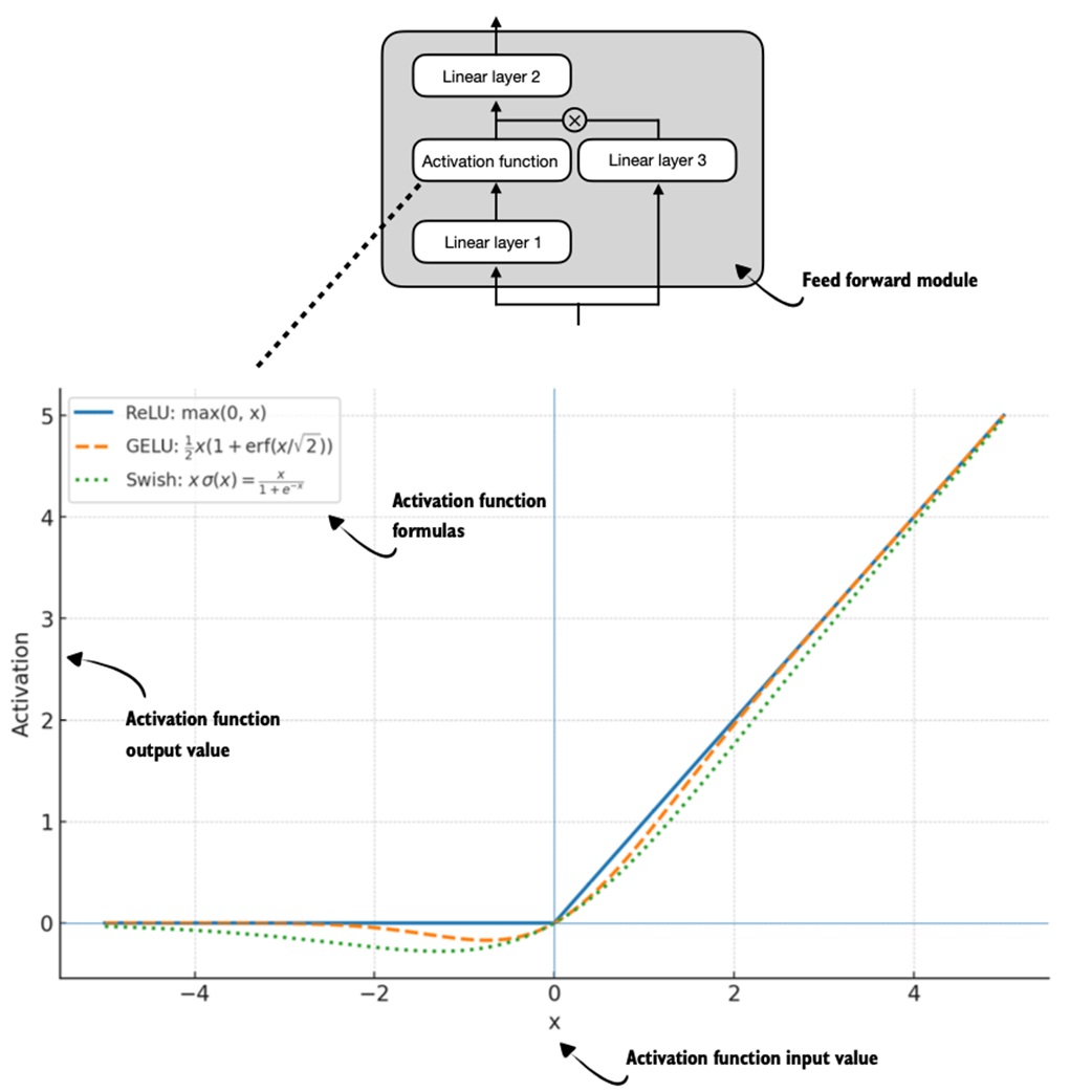 Figure C.4 Different activation functions that can be used in a feed forward module (neural network). GELU and SiLU (Swish) offer smooth alternatives to ReLU, which has a sharp kink at input zero.
GELU involves the Gaussian cumulative distribution function (CDF). Computing this CDF is slow because it uses piecewise logic and exponentials, which makes it hard to write fused, optimized GPU kernels (although a fast approximation exists that uses cheaper operations and runs faster with near-identical results).
In short, while GELU produces smooth activation curves, it is overall computationally more expensive than simpler functions.
Newer models have largely replaced GELU with the SiLU (also known as Swish) function, which smoothly suppresses large negative inputs toward ~0 and is approximately linear for large positive inputs, as shown in figure C.4.
SiLU has a similar smoothness, but it is slightly cheaper to compute than GELU and offers comparable modeling performance. In practice, SiLU is now used in most architectures, while GELU remains in use in only some models, such as Google’s Gemma open-weight LLM. In the implementation of the feed forward module in listing C.2, this SiLU function is called via nn.functional.silu. The feed forward module in listing C.2 is also often called SwiGLU, an abbreviation that is derived from the terms Swish and GLU.
C.3 Rotary position embeddings (RoPE)
In transformer-based LLMs, positional encoding is necessary because of the attention mechanism. By default, attention treats the input tokens as if they have no order. In the original GPT architecture, absolute positional embeddings addressed this by adding a learned embedding vector for each position in the sequence, which is then added to the token embedding.
RoPE (short for rotary position embeddings) introduced a different approach: instead of adding position information as separate embeddings, it encodes position information by rotating the query and key vectors in the attention mechanism (section C.4) in a way that depends on each token’s position. RoPE is an elegant idea, but also a long topic in itself. Interested readers can find more information in the original RoPE paper at https://arxiv.org/abs/2104.09864. (While first introduced in 2021, RoPE became widely adopted with the release of the original Llama model in 2023 and has since become a staple in modern LLMs, so it is not unique to Qwen3.)
RoPE can be implemented in two mathematically equivalent ways: the interleaved form, which pairs adjacent dimensions for rotation, or in a two-halves form, which splits the dimension into cosine and sine halves for convenience. Listing C.3 implements the two-halves variant, which can be easier to read.
Listing C.3 RoPE functions
import torch


def compute_rope_params(head_dim, theta_base=10_000, context_length=4096,
                        dtype=torch.float32):
    assert head_dim % 2 == 0, "Embedding dimension must be even"
    inv_freq = 1.0 / (theta_base ** (
        torch.arange(0, head_dim, 2, dtype=dtype)[: (head_dim // 2)].float()
        / head_dim
    ))
    positions = torch.arange(context_length, dtype=dtype)
    angles = positions.unsqueeze(1) * inv_freq.unsqueeze(0)
    angles = torch.cat([angles, angles], dim=1)

    cos = torch.cos(angles)
    sin = torch.sin(angles)

    return cos, sin


def apply_rope(x, cos, sin, offset=0):
    # The shape is (batch_size, num_heads, seq_len, head_dim)
    batch_size, num_heads, seq_len, head_dim = x.shape
    assert head_dim % 2 == 0, "Head dimension must be even"

    # Split x into first half and second half
    x1 = x[..., : head_dim // 2]  # First half
    x2 = x[..., head_dim // 2:]  # Second half

    cos = cos[offset:offset + seq_len, :].unsqueeze(0).unsqueeze(0)
    sin = sin[offset:offset + seq_len, :].unsqueeze(0).unsqueeze(0)
    # Shape after:  (1, 1, seq_len, head_dim)

    rotated = torch.cat((-x2, x1), dim=-1)
    # It's ok to use lower-precision after applying cos and sin rotation
    x_rotated = (x * cos) + (rotated * sin)

    return x_rotated.to(dtype=x.dtype)
The RoPE code in listing C.3 will be used in the grouped query attention mechanism in section C.4.
RoPE implementation variants
Readers familiar with the original RoPE paper (https://arxiv.org/abs/2104.09864), you may be wondering about the particular implementation I have chosen.
There are two common styles to implement RoPE, which are mathematically equivalent. The implementations mainly differ in how the rotation matrix pairs dimensions. I chose the split-halves style as it is a bit easier to read and implement.
1) Split-halves style (this book, Hugging Face Transformers):
[ x0   x1   x2   x3   x4   x5   x6   x7 ]
  │    │    │    │    │    │    │    │
  ▼    ▼    ▼    ▼    ▼    ▼    ▼    ▼
 cos  cos  cos  cos  sin  sin  sin  sin
Rotation matrix:
[ cosθ   -sinθ    0      0   ... ]
[ sinθ    cosθ    0      0   ... ]
[  0       0    cosθ   -sinθ ... ]
[  0       0    sinθ    cosθ ... ]
Here, the embedding dimensions are split into two halves and then each one is rotated in blocks.
2) Interleaved (even/odd) style (original paper, Llama repo):
[ x0   x1   x2   x3   x4   x5   x6   x7 ]
  │    │    │    │    │    │    │    │
  ▼    ▼    ▼    ▼    ▼    ▼    ▼    ▼
 cos  sin  cos  sin  cos  sin  cos  sin
Rotation matrix:
[ cosθ  -sinθ    0      0   ... ]
[ sinθ   cosθ    0      0   ... ]
[  0      0    cosθ   -sinθ ... ]
[  0      0    sinθ    cosθ ... ]
Here, embedding dims are interleaved as even/odd cosine/sine pairs. Both styles encode the same relative position. The only difference is how dimensions are paired.
C.4 Grouped query attention (GQA)
Grouped query attention (GQA) has become the standard, more compute- and parameter-efficient alternative to the original multi-head attention (MHA) mechanism.
Unlike MHA, where each head has its own set of keys and values, to reduce memory usage, GQA groups multiple heads to share the same key and value projection, as shown in figure C.5.
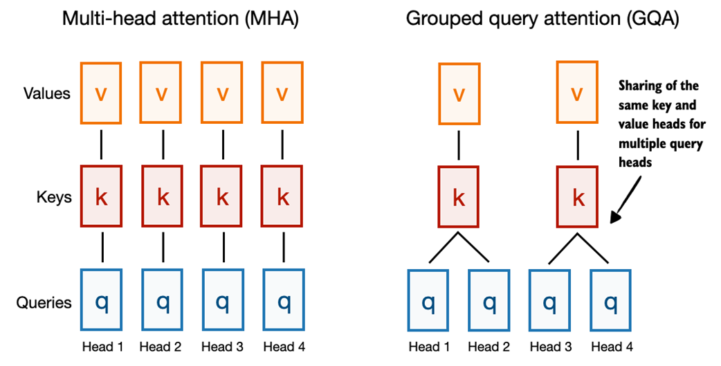 Figure C.5 A comparison between MHA and GQA. Here, the group size is 2, where a key and value pair is shared among 2 queries.
So, the core idea behind GQA, shown in figure C.5, is to reduce the number of key and value heads by sharing them across multiple query heads. This (1) lowers the model’s parameter count and (2) reduces the memory bandwidth usage for key and value tensors during inference since fewer keys and values need to be stored and retrieved from the KV cache (section C.7).
While GQA is primarily a computational efficiency workaround for MHA, ablation studies (as presented in the original GQA paper, https://arxiv.org/abs/2305.13245) show that it performs comparably to standard MHA in terms of LLM modeling performance.
Listing C.4 implements the GQA mechanism with KV cache support.
Listing C.4 Grouped query attention
class GroupedQueryAttention(nn.Module):
    def __init__(self, d_in, num_heads, num_kv_groups, head_dim=None,
                 qk_norm=False, dtype=None):
        super().__init__()
        assert num_heads % num_kv_groups == 0

        self.num_heads = num_heads
        self.num_kv_groups = num_kv_groups
        self.group_size = num_heads // num_kv_groups

        if head_dim is None:
            assert d_in % num_heads == 0
            head_dim = d_in // num_heads

        self.head_dim = head_dim
        self.d_out = num_heads * head_dim

        self.W_query = nn.Linear(
            d_in, self.d_out, bias=False, dtype=dtype
        )
        self.W_key = nn.Linear(
            d_in, num_kv_groups * head_dim, bias=False,dtype=dtype
        )
        self.W_value = nn.Linear(
            d_in, num_kv_groups * head_dim, bias=False, dtype=dtype
        )

        self.out_proj = nn.Linear(self.d_out, d_in, bias=False, dtype=dtype)

        if qk_norm:
            self.q_norm = RMSNorm(head_dim, eps=1e-6)
            self.k_norm = RMSNorm(head_dim, eps=1e-6)
        else:
            self.q_norm = self.k_norm = None

    def forward(self, x, mask, cos, sin, start_pos=0, cache=None):
        b, num_tokens, _ = x.shape

        # The shape is (b, num_tokens, num_heads * head_dim)
        queries = self.W_query(x)
        # The shapes are (b, num_tokens, num_kv_groups * head_dim)
        keys = self.W_key(x)
        values = self.W_value(x)

        queries = queries.view(b, num_tokens, self.num_heads,
                               self.head_dim).transpose(1, 2)
        keys_new = keys.view(b, num_tokens, self.num_kv_groups,
                             self.head_dim).transpose(1, 2)
        values_new = values.view(b, num_tokens, self.num_kv_groups,
                                 self.head_dim).transpose(1, 2)

        if self.q_norm:
            queries = self.q_norm(queries)
        if self.k_norm:
            keys_new = self.k_norm(keys_new)

        queries = apply_rope(queries, cos, sin, offset=start_pos)
        keys_new = apply_rope(keys_new, cos, sin, offset=start_pos)

        if cache is not None:
            prev_k, prev_v = cache
            keys = torch.cat([prev_k, keys_new], dim=2)
            values = torch.cat([prev_v, values_new], dim=2)
        else:
            # Reset RoPE
            start_pos = 0
            keys, values = keys_new, values_new
        next_cache = (keys, values)

        # Expand K and V to match number of heads
        keys = keys.repeat_interleave(
            self.group_size, dim=1
        )
        values = values.repeat_interleave(
            self.group_size, dim=1
        )

        attn_scores = queries @ keys.transpose(2, 3)
        attn_scores = attn_scores.masked_fill(mask, -torch.inf)
        attn_weights = torch.softmax(
            attn_scores / self.head_dim**0.5, dim=-1
        )

        context = (attn_weights @ values).transpose(1, 2)
        context = context.reshape(b, num_tokens, self.d_out)
        return self.out_proj(context), next_cache
You may also have noticed that the GQA mechanism in listing C.4 also includes a qk_norm parameter. This is not part of the standard GQA design. When qk_norm=True, an additional Query/Key-RMSNorm-based normalization, called QKNorm, is applied to both the queries and keys, which is a technique used in Qwen3. As discussed earlier in the RMSNorm section (section C.1), QKNorm helps improve training stability.
C.5 Transformer block
The transformer block is the central component of an LLM, which combines all the individual elements covered in this appendix so far. As shown in figure C.6, it is repeated multiple times; in the 0.6-billion-parameter version of Qwen3, it is repeated 28 times.
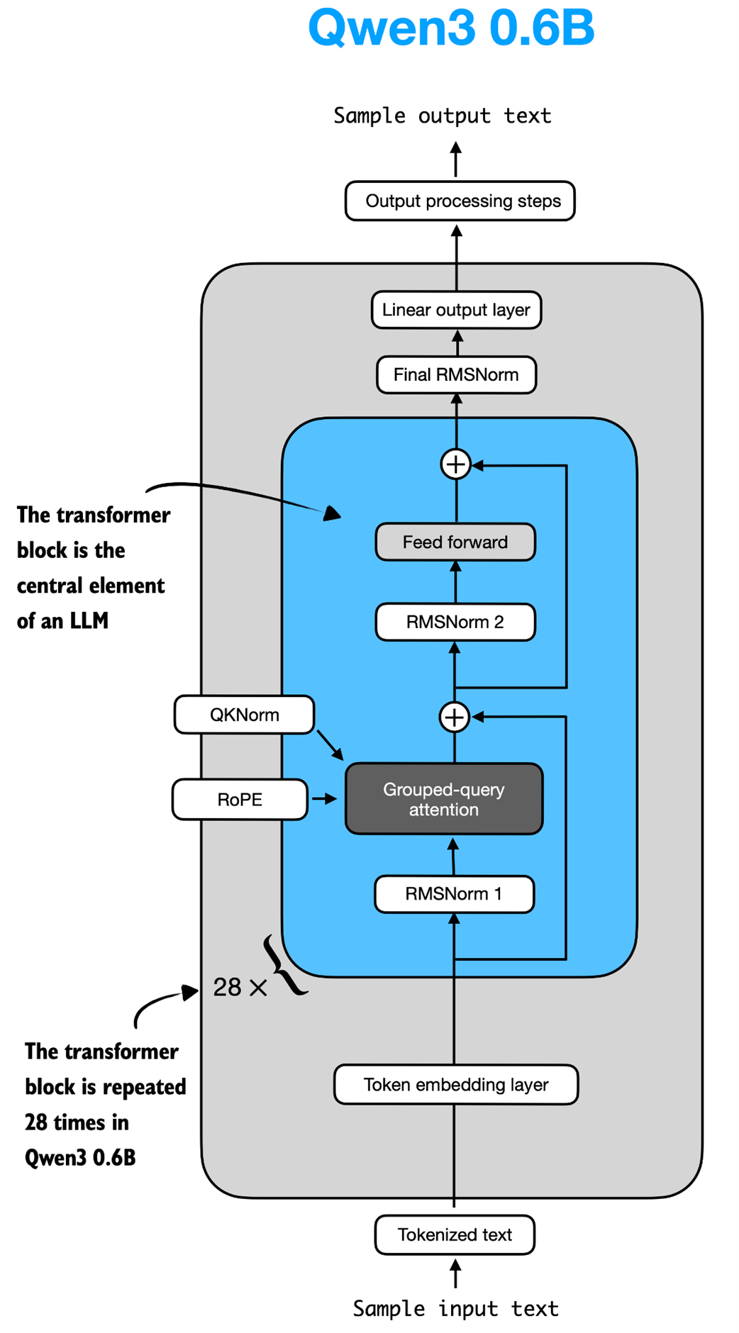 Figure C.6 The Structure of the transformer block in Qwen3. Each block includes RMSNorm, RoPE, masked grouped-query attention, and a feed-forward module, and is repeated 28 times in the 0.6B-parameter model.
Listing C.5 implements the transformer block shown in figure C.6.
Listing C.5 Transformer block
class TransformerBlock(nn.Module):
    def __init__(self, cfg):
        super().__init__()
        self.att = GroupedQueryAttention(
            d_in=cfg["emb_dim"],
            num_heads=cfg["n_heads"],
            head_dim=cfg["head_dim"],
            num_kv_groups=cfg["n_kv_groups"],
            qk_norm=cfg["qk_norm"],
            dtype=cfg["dtype"]
        )
        self.ff = FeedForward(cfg)
        self.norm1 = RMSNorm(cfg["emb_dim"], eps=1e-6)
        self.norm2 = RMSNorm(cfg["emb_dim"], eps=1e-6)

    def forward(self, x, mask, cos, sin, start_pos=0, cache=None):
        shortcut = x
        x = self.norm1(x)
        # The shape is (batch_size, num_tokens, emb_size)
        x, next_cache = self.att(
            x, mask, cos, sin, start_pos=start_pos,cache=cache
        )
        x = x + shortcut

        shortcut = x
        x = self.norm2(x)
        x = self.ff(x)
        x = x + shortcut

        return x, next_cache
As we can see, in listing C.5, the transformer block simply connects various elements we implemented in previous sections.
C.6 Main model code
In this section, we will define the Qwen3Model class that we imported and used in chapter 2.
To implement the Qwen3Model class, the code in listing C.6 follows the architecture previously shown in figure C.6, where the transformer block sits at the heart of the LLM.
Listing C.6 Main Qwen3Model code
class Qwen3Model(nn.Module):
    def __init__(self, cfg):
        super().__init__()

        # Main model parameters
        self.tok_emb = nn.Embedding(cfg["vocab_size"], cfg["emb_dim"],
                                    dtype=cfg["dtype"])

        self.trf_blocks = nn.ModuleList(
            [TransformerBlock(cfg) for _ in range(cfg["n_layers"])]
        )
        self.final_norm = RMSNorm(cfg["emb_dim"])
        self.out_head = nn.Linear(
            cfg["emb_dim"], cfg["vocab_size"],
            bias=False, dtype=cfg["dtype"]
        )

        # Reusable utilities
        if cfg["head_dim"] is None:
            head_dim = cfg["emb_dim"] / cfg["n_heads"]
        else:
            head_dim = cfg["head_dim"]
        cos, sin = compute_rope_params(
            head_dim=head_dim,
            theta_base=cfg["rope_base"],
            context_length=cfg["context_length"]
        )
        self.register_buffer("cos", cos, persistent=False)
        self.register_buffer("sin", sin, persistent=False)
        self.cfg = cfg
        self.current_pos = 0  # Track current position in KV cache

    def forward(self, in_idx, cache=None):
        tok_embeds = self.tok_emb(in_idx)
        x = tok_embeds

        num_tokens = x.shape[1]
        if cache is not None:
            pos_start = self.current_pos
            pos_end = pos_start + num_tokens
            self.current_pos = pos_end
            mask = torch.triu(
                torch.ones(
                    pos_end, pos_end, device=x.device, dtype=torch.bool
                ),
                diagonal=1
            )[pos_start:pos_end, :pos_end]
        else:
            pos_start = 0  # Not strictly necessary but helps torch.compile
            mask = torch.triu(
                torch.ones(num_tokens, num_tokens, device=x.device,
                           dtype=torch.bool),
                diagonal=1
            )

        # Prefill: Shape (1, 1, T, T) to broadcast across batch and heads.
        # Cached: Shape (1, 1, T, K+T) where T=new tokens, K=cached keys.
        mask = mask[None, None, :, :]

        for i, block in enumerate(self.trf_blocks):
            blk_cache = cache.get(i) if cache else None
            x, new_blk_cache = block(x, mask, self.cos, self.sin,
                                     start_pos=pos_start,
                                     cache=blk_cache)
            if cache is not None:
                cache.update(i, new_blk_cache)

        x = self.final_norm(x)
        logits = self.out_head(x.to(self.cfg["dtype"]))
        return logits

    def reset_kv_cache(self):
        self.current_pos = 0
Since we already have all the main ingredients, the Qwen3Model class in listing C.6 only adds a few more components around the transformer block, namely the embedding and output layers (including one more RMSNorm layer). However, the code may appear somewhat complicated, which is due to the KV cache option.
As discussed in chapter 2, the KV cache can speed up the text generation process, but it is a topic outside the scope of this book. Interested readers can find more information about KV caching in my Understanding and Coding the KV Cache in LLMs from Scratch article at https://magazine.sebastianraschka.com/p/coding-the-kv-cache-in-llms.
Note that the Qwen3Model class, as implemented in listing C.6, supports various model sizes (see appendix D for more information). In chapter 2, we use the 0.6-billion-parameter model as it is the least resource-intensive model in the Qwen3 model family. The specific configuration of this model is visualized in figure C.7.
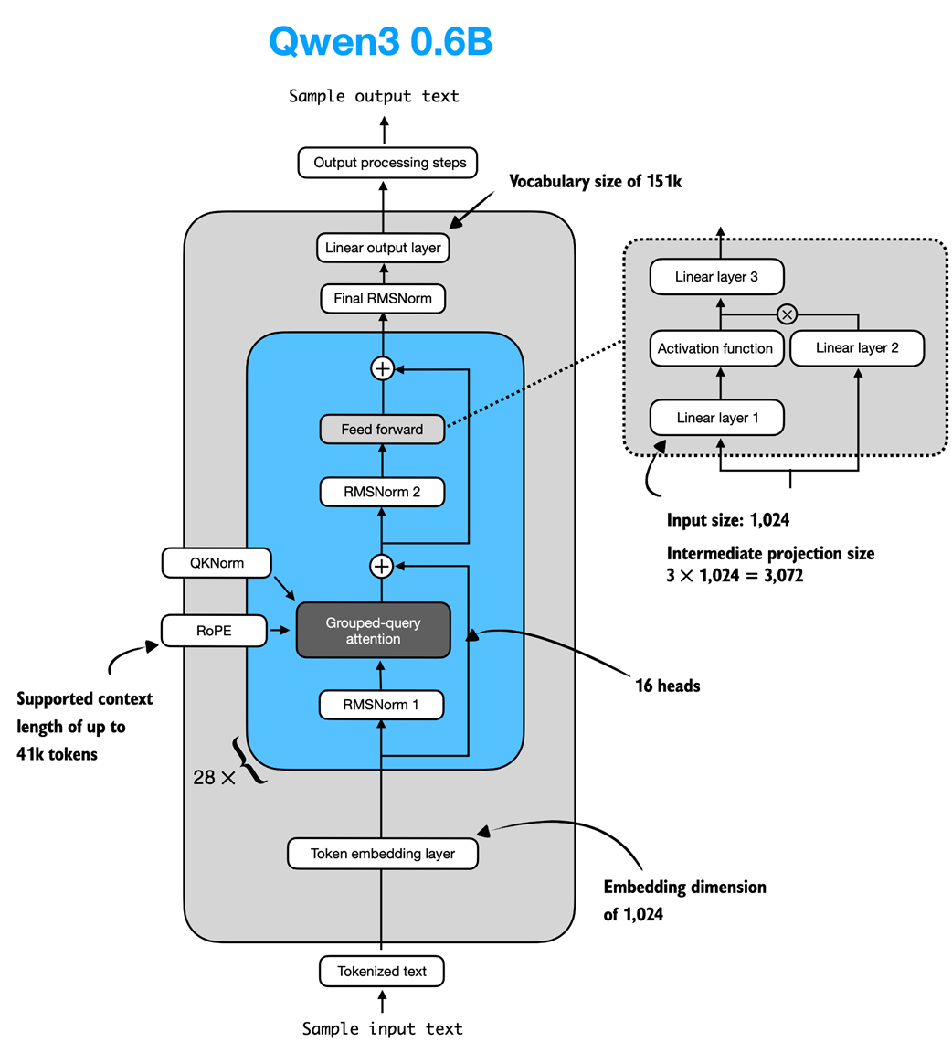 Figure C.7 Architecture of the Qwen3 0.6B model. The model consists of a token embedding layer followed by 28 transformer blocks, each containing RMSNorm, RoPE, QKNorm, masked grouped-query attention with 16 heads, and a feed-forward module with an intermediate size of 3,072.
To use the 0.6B model shown in figure C.7 via the Qwen3Model class, we can define the following configuration in listing C.7 that we provide as input (cfg=QWEN_CONFIG_06_B) upon instantiating a new Qwen3Model instance.
Listing C.7 Qwen3 0.6B configuration
QWEN_CONFIG_06_B = {
    "vocab_size": 151_936,     # Vocabulary size
    "context_length": 40_960,  # Length originally used during training
    "emb_dim": 1024,           # Embedding dimension
    "n_heads": 16,             # Number of attention heads
    "n_layers": 28,            # Number of layers
    "hidden_dim": 3072,        # Size of intermediate dim in FeedForward
    "head_dim": 128,           # Size of the heads in GQA
    "qk_norm": True,           # Whether to normalize queries & keys in GQA
    "n_kv_groups": 8,          # Key-Value groups for GQA
    "rope_base": 1_000_000.0,  # The base in RoPE's "theta"
    "dtype": torch.bfloat16,   # Lower-precision dtype to reduce memory
}
We will use the QWEN_CONFIG_06_B configuration from listing C.7 to instantiate the Qwen3 0.6B model later in section C.9.
More Precise Context Length Information
For Qwen3 0.6B, the default maximum supported context length is 40,960 tokens. However, the model itself was trained with only 32,768 tokens. The 40,960-token allocation reserves 32,768 tokens for model outputs (the generated text) and 8,192 tokens for typical prompts (the users’ question or instructions).
To put this in perspective, 40 thousand tokens corresponds to roughly one half of the first Harry Potter book.
Since this length is sufficient for most reasoning tasks, the developers note that context-extension methods (such as YaRN) are not recommended unless the average context regularly exceeds 32 thousand tokens, as enabling them in shorter contexts can slightly degrade performance.
C.7 KV cache
The KV-cache-related heavy-lifting is mostly done in the Qwen3Model (listing C.6) and GroupedQueryAttention (listing C.4) code. The KVCache, shown in listing C.8, stores the key-value pairs themselves during text generation, which results in the speedup we experienced when enabling KV caching in chapter 2.
Listing C.8 KV Cache
class KVCache:
    def __init__(self, n_layers):
        self.cache = [None] * n_layers

    def get(self, layer_idx):
        return self.cache[layer_idx]

    def update(self, layer_idx, value):
        self.cache[layer_idx] = value

    def get_all(self):
        return self.cache

    def reset(self):
        for i in range(len(self.cache)):
            self.cache[i] = None
The KVCache class in listing C.8 is used inside the generate_text_basic_cache function that we implemented in chapter 2.
C.8 Tokenizer
The tokenizer code is somewhat complicated, as it supports a variety of special tokens, in addition to the base model and the so-called “Thinking” model variant of Qwen3, which is a reasoning model. The full implementation of the tokenizer is shown in listing C.9.
Listing C.9 Tokenizer
import re
from tokenizers import Tokenizer

class Qwen3Tokenizer:
    _SPECIALS = [
        "<|endoftext|>",
        "<|im_start|>", "<|im_end|>",
        "<|object_ref_start|>", "<|object_ref_end|>",
        "<|box_start|>", "<|box_end|>",
        "<|quad_start|>", "<|quad_end|>",
        "<|vision_start|>", "<|vision_end|>",
        "<|vision_pad|>", "<|image_pad|>", "<|video_pad|>",
    ]
    _SPLIT_RE = re.compile(r"(<\|[^>]+?\|>)")

    def __init__(self,
                 tokenizer_file_path="tokenizer-base.json",
                 apply_chat_template=False,
                 add_generation_prompt=False,
                 add_thinking=False):

        self.apply_chat_template = apply_chat_template
        self.add_generation_prompt = add_generation_prompt
        self.add_thinking = add_thinking

        tok_path = Path(tokenizer_file_path)
        if not tok_path.is_file():
            # Match HF behavior: chat model: <|im_end|>, base model: <|endoftext|>
            raise FileNotFoundError(
                f"Tokenizer file '{tok_path}' not found. "
            )

        self._tok = Tokenizer.from_file(str(tok_path))
        self._special_to_id = {t: self._tok.token_to_id(t)
                               for t in self._SPECIALS}

        self.pad_token = "<|endoftext|>"
        self.pad_token_id = self._special_to_id.get(self.pad_token)

        f = tok_path.name.lower()
        if "base" in f and "reasoning" not in f:
            self.eos_token = "<|endoftext|>"
        else:
            self.eos_token = "<|im_end|>"
        self.eos_token_id = self._special_to_id.get(self.eos_token)

    def encode(self, prompt, chat_wrapped=None):
        if chat_wrapped is None:
            chat_wrapped = self.apply_chat_template

        stripped = prompt.strip()
        if stripped in self._special_to_id and "\n" not in stripped:
            return [self._special_to_id[stripped]]

        if chat_wrapped:
            prompt = self._wrap_chat(prompt)

        ids = []
        for part in filter(None, self._SPLIT_RE.split(prompt)):
            if part in self._special_to_id:
                ids.append(self._special_to_id[part])
            else:
                ids.extend(self._tok.encode(part).ids)
        return ids

    def decode(self, token_ids):
        return self._tok.decode(token_ids, skip_special_tokens=False)

    def _wrap_chat(self, user_msg):
        s = f"<|im_start|>user\n{user_msg}<|im_end|>\n"
        if self.add_generation_prompt:
            s += "<|im_start|>assistant"
            if self.add_thinking:
                # insert no <think> tag, just a new line
                s += "\n"
            else:
                s += "\n<think>\n\n</think>\n\n"
        return s
Note that our Qwen3Tokenizer implementation in listing C.9 may appear somewhat complicated, as it aims to replicate the behavior of the official tokenizer released by the Qwen3 team in the Hugging Face Transformers library.
At first glance, it appears to have a few quirks. For example, when add_thinking=True, no "\n<think>\n\n</think>\n\n" tokens are inserted (where \n is a newline character), and when add_thinking=False, these tokens are added. This is intentional because the non-base Qwen3 0.6B model is a hybrid that supports both reasoning (“thinking”) and standard modes.
C.9 Using the model
Let’s now instantiate and use the model to confirm that the code works by reusing the text generation approach from chapter 2.
First, we instantiate the model using the pre-trained model weights:
from pathlib import Path
import torch

from reasoning_from_scratch.ch02 import get_device
from reasoning_from_scratch.qwen3 import download_qwen3_small

# Optional: Uncomment to use automatic device picker
# device = get_device()
device = torch.device("cpu")

download_qwen3_small(kind="base", tokenizer_only=False, out_dir="qwen3")

tokenizer_file_path = Path("qwen3") / "tokenizer-base.json"
model_file = Path("qwen3") / "qwen3-0.6B-base.pth"

tokenizer = Qwen3Tokenizer(tokenizer_file_path=tokenizer_file_path)
model = Qwen3Model(QWEN_CONFIG_06_B)
model.load_state_dict(torch.load(model_file))

model.to(device)
The output shows the structure of the instantiated model, which should match the values we used in the configuration file in listing C.7:
✓ qwen3/qwen3-0.6B-base.pth already up-to-date
✓ qwen3/tokenizer-base.json already up-to-date
Qwen3Model(
  (tok_emb): Embedding(151936, 1024)
  (trf_blocks): ModuleList(
    (0-27): 28 x TransformerBlock(
      (att): GroupedQueryAttention(
        (W_query): Linear(in_features=1024, out_features=2048, bias=False)
        (W_key): Linear(in_features=1024, out_features=1024, bias=False)
        (W_value): Linear(in_features=1024, out_features=1024, bias=False)
        (out_proj): Linear(in_features=2048, out_features=1024, bias=False)
        (q_norm): RMSNorm()
        (k_norm): RMSNorm()
      )
      (ff): FeedForward(
        (fc1): Linear(in_features=1024, out_features=3072, bias=False)
        (fc2): Linear(in_features=1024, out_features=3072, bias=False)
        (fc3): Linear(in_features=3072, out_features=1024, bias=False)
      )
      (norm1): RMSNorm()
      (norm2): RMSNorm()
    )
  )
  (final_norm): RMSNorm()
  (out_head): Linear(in_features=1024, out_features=151936, bias=False)
)
Next, we re-use the text generation functions from chapter 2 to generate text:
import time

from reasoning_from_scratch.ch02 import (
    generate_stats,
    generate_text_basic_cache,
)

prompt = "Explain large language models in a single sentence."

input_token_ids_tensor = torch.tensor(
    tokenizer.encode(prompt),
    device=device
    ).unsqueeze(0)

start_time = time.time()

output_token_ids_tensor = generate_text_basic_cache(
    model=model,
    token_ids=input_token_ids_tensor,
    max_new_tokens=200,
    eos_token_id=tokenizer.eos_token_id,
)
end_time = time.time()

generate_stats(output_token_ids_tensor, tokenizer, start_time, end_time)
Since we used the same prompt as in chapter 2, the generated text matches the generated text from chapter 2 exactly:
Time: 1.46 sec
28 tokens/sec

 Large language models are artificial intelligence systems that can
understand, generate, and process human language, enabling them to
perform a wide range of tasks, from answering questions to writing
articles, and even creating creative content.
While the main chapters use the 0.6-billion-parameter variant of Qwen3 to lower the resource requirements for this book, interested readers can find more information on how to use the larger models in appendix D.