Exercise solutions
Appendix B. Exercise solutions
The complete code examples for the exercise solutions can be found in the supplementary GitHub repository at https://github.com/rasbt/reasoning-from-scratch.
B.1 Chapter 2
Exercise 2.1
We can use a prompt similar to “Hello, Ardwarklethyrx. Haus und Garten.”, which contains a made-up word ("Ardwarklethyrx") and three words in a non-English language (German):
prompt = "Hello, Ardwarklethyrx. Haus und Garten."
input_token_ids_list = tokenizer.encode(prompt)
for i in input_token_ids_list:
    print(f"{[i]} --> {tokenizer.decode([i])}")
The output is:
[9707] --> Hello
[11] --> ,
[1644] -->  Ar
[29406] --> dw
[838] --> ark
[273] --> le
[339] --> th
[10920] --> yr
[87] --> x
[13] --> .
[47375] -->  Haus
[2030] -->  und
[93912] -->  Garten
[13] --> .
As we can see, unknown words are broken into smaller pieces of subwords or even single tokens; this allows the tokenizer and LLM to handle any input.
German words are not broken down into characters or even subwords here, suggesting that the tokenizer has seen German texts during training. This also suggests that the LLM was likely trained on German texts, too, and should be able to handle at least certain non-English languages well.
Exercise 2.2
We can simply delete the line device = torch.device("cpu") in section 2.5, and then rerun the rest of the code in chapter 2 as is. Reference numbers for the hardware I tried the code on are provided in table 2.1 at the end of chapter 2.
B.2 Chapter 3
Exercise 3.1
There is an endless number of different test cases we may add. Below is a selection of some interesting ones:
from reasoning_from_scratch.ch03 import (
    run_demos_table
)

more_tests = [
    ("check_17", "[1, 2]", "(1, 2)", True),  # A: Different bracket types
    ("check_18", "1e-3", "0.001", True),     # B: Scientific notation
    ("check_19", "(-3)^2", "9", True),      # C: Algebraic simplification with caret exponent
    ("check_20", "−1", "-1", True),          # D: Unicode minus (U+2212) vs ASCII hyphen-minus
]
run_demos_table(more_tests)
The output is:
Test     | Expect | Got   | Status
check_17 | True   | True  | PASS
check_18 | True   | True  | PASS
check_19 | True   | True  | PASS
check_20 | True   | False | FAIL
As we can see, the test fails for check_20, which uses the Unicode version of a minus sign that looks indistinguishable to the human eye (depending on which font or editor you use). We could fix this test case by adding one of the following lines anywhere in the normalize_text function:
text = text.replace("−", "-")
or
text = text.replace("\u2212", "-")
Another interesting test is the following one:
extra_tests_1 = [
    ("check_21", "Text around answer 3.", "3", True)
]
We can run it via the following code:
run_demos_table(extra_tests_1)
However, it fails the test:
Test     | Expect | Got   | Status
check_21 | True   | False | FAIL

Passed 0/1
Note that this might look like an issue with the grading logic at first, but it is actually a poorly designed test. In practice, the run_demos_table function is intended specifically to test the grade_answer function; nothing more, nothing less.
The grade_answer function would never receive the entire answer in this text form, since the answer would have been extracted from the text before being passed to it. For instance, if we want to test text answers, we need to call the test as follows:
from reasoning_from_scratch.ch03 import (
    extract_final_candidate
)
extra_tests_2 = [
    ("check_21",
     extract_final_candidate("Text around answer 3."),
     "3", True)
]
As we can see based on the output, it now passes the test:
run_demos_table(extra_tests_2)
Test     | Expect | Got  | Status
check_21 | True   | True | PASS

Passed 1/1
Exercise 3.2
There are two options to calculate the average response length. The first option is to modify the evaluate_math500_stream function (listing 3.13 in chapter 3) by adding the following lines:
# ...
# below `num_correct = 0`
total_len = 0

# ...
# inside for i, row in enumerate(math_data, start=1):
# anywhere below `gen_text = ...`
total_len += len(tokenizer.encode(gen_text))

# ...
# anywhere at the bottom before the return statement
avg_len = total_len / num_examples
print(f"Average length: {avg_len:.2f} tokens")
Alternatively, the second option is to calculate the response lengths from the .jsonl files that were created when we ran the evaluate_math500_stream function in the main chapter. This way, we avoid having to rerun the evaluation.
First, we load the .jsonl file as follows:
import json
from pathlib import Path

WHICH_MODEL = "base"
dev_name = "mps"

# A: You may need to adjust this path
local_path = Path(f"math500-{dev_name}.jsonl")
if not local_path.exists():
    raise FileNotFoundError(
        f"{local_path} not found. Run ch03_main.ipynb to create it."
    )

results = []
with open(local_path, "r") as f:
    for line in f:
        if line.strip():
            results.append(json.loads(line))

print("Number of entries:", len(results))
Let’s print the dictionary keys to get a better idea of how the results dataset is structured:
print(results[0].keys())
This prints:
dict_keys(['index', 'problem', 'gtruth_answer', 'generated_text', 'extracted', 'correct'])
Each item contains multiple keys; however, we are only interested in the "generated_text" key, which contains the model’s full answer. Next, we need to load the tokenizer so that we can tokenize the answer text before we can calculate the number of tokens. This is similar to the code we used in listing 3.1 in chapter 3:
from reasoning_from_scratch.qwen3 import (
    download_qwen3_small,
    Qwen3Tokenizer
)

if WHICH_MODEL == "base":
    download_qwen3_small(
        kind="base", tokenizer_only=True, out_dir="qwen3"
    )
    tokenizer_path = Path("qwen3") / "tokenizer-base.json"
    tokenizer = Qwen3Tokenizer(tokenizer_file_path=tokenizer_path)

elif WHICH_MODEL == "reasoning":
    download_qwen3_small(
        kind="reasoning", tokenizer_only=True, out_dir="qwen3"
    )
    tokenizer_path = Path("qwen3") / "tokenizer-reasoning.json"
    tokenizer = Qwen3Tokenizer(
        tokenizer_file_path=tokenizer_path,
        apply_chat_template=True,
        add_generation_prompt=True,
        add_thinking=True,
    )
Then, we can calculate the average length as follows, which is similar to how we could have modified the evaluate_math500_stream function:
total_len = 0

for item in results:
    num_tokens = len(tokenizer.encode(item["generated_text"]))
    total_len += num_tokens

avg_len = total_len / len(results)
print(f"Average length: {avg_len:.2f} tokens")
The resulting average length is as follows:
Average length: 98.00 tokens
Table B.1 lists the average lengths for the different models and subsets.
Table B.1 Average number of tokens on MATH-500
| Model | Device | Average length | MATH-500 size |
|---|---|---|---|
| Base | CPU | 97.30 | 10 |
| Base | CUDA | 96.74 | 500 |
| Reasoning | CPU | 891.80 | 10 |
| Reasoning | CUDA | 1361.21 | 500 |
As we can see based on the results in table B.1, and as expected, the reasoning model generates much longer responses (in this case, approximately 10-times longer).
Exercise 3.3
To evaluate the model on a larger dataset, we can simply change the math_data[:10] to a different slice or larger number (up to 500) in the following function call:
num_correct, num_examples, acc = evaluate_math500_stream(
    model, tokenizer, device,
    math_data=math_data[:10],
    max_new_tokens=2048,
    verbose=False
)
Table B.2 below shows the accuracy values for different dataset sizes. (Since the MATH-500 test set is already shuffled, no additional shuffling was applied.)
Table B.2 Accuracies for different MATH-500 dataset sizes
| Model | Device | Accuracy | MATH-500 size |
|---|---|---|---|
| Base | CUDA | 30.0% | 10 |
| Base | CUDA | 34.0% | 50 |
| Base | CUDA | 27.0% | 100 |
| Base | CUDA | 15.3% | 500 |
| Reasoning | CUDA | 90.0% | 10 |
| Reasoning | CUDA | 58.0% | 50 |
| Reasoning | CUDA | 56.0% | 100 |
| Reasoning | CUDA | 48.2% | 500 |
As we can see based on the results in table B.2, the first 10 examples are not very representative of the MATH-500 performance evaluated on the whole 500 examples.
In addition, we can create an entirely new dataset in a similar style to MATH-500. For example, a dataset in MATH-500 style is included in this repository; we can use it in the main chapter by changing the filename from math500_test.json to math_new50_exercise.json (this dataset is included in this book’s GitHub repository at https://github.com/rasbt/reasoning-from-scratch/tree/main/ch03/01_main-chapter-code).
The performance of the models is as follows:
- Base: 36.0% (18/50)
- Reasoning: 80.0% (40/50)
Accuracy is similar for the base model and higher for the reasoning model compared to the 50-example subset of the MATH-500 test set (table B.2). This indicates that, despite the possibility of overlap with Qwen3’s training data, the model generalizes well to new math questions and does not show signs of extensive overfitting to the original MATH-500 data.
Exercise 3.4
We could use the alternative prompt similar to the one suggested in the chapter, which modifies the prompt to use the word “problem” instead of “question”:
def render_prompt(prompt):
    template = (
        "You are a helpful math assistant.\n"
        "Solve the problem and write the final "
        "result on a new line as:\n"
        "\\boxed{ANSWER}\n\n"
        f"Problem:\n{prompt}\n\nAnswer:"
    )
    return template
Using this prompt improves the performance of the base model, on the 500 examples, from 15.3% to 31.2%. Also, it improves the performance of the reasoning model from 48.2% to 50.0%.
From these observations, we may conclude that the base model is much more sensitive to the prompt format (likely due to memorizing some prompt-formatted MATH-500 examples from the training set) than the reasoning model; the latter seems largely unaffected.
B.3 Chapter 4
Exercise 4.1
The modification only requires adding a prompt suffix such as "\n\nExplain step by step." after applying the prompt template. There is only a very small portion of code that needs to be updated in the MATH-500 evaluation function from chapter 3, as shown below:
def evaluate_math500_stream(...):
    # ...
        for i, row in enumerate(math_data, start=1):
            prompt = render_prompt(row["problem"])
            prompt += "\n\nExplain step by step."  # NEW
            gen_text = generate_text_stream_concat(
                model, tokenizer, prompt, device,
                max_new_tokens=max_new_tokens,
                verbose=verbose,
            )
     # ...
The improvements are shown in row 3 in table 4.1, which can be found in section 4.6 in chapter 4.
Exercise 4.2
Here, we replace the generate_text_stream_concat function with generate_text_stream_concat_flex and pass in generate_text_top_p_stream_cache as its generation function. The updated MATH-500 evaluation function from chapter 3 is shown below, and the changes are marked with comments labeled # NEW.
def evaluate_math500_stream(
    model,
    tokenizer,
    device,
    math_data,
    out_path=None,
    max_new_tokens=512,
    verbose=False,
    temperature=1.0,  # NEW
    top_p=1.0,        # NEW
):
    # ...
    with open(out_path, "w", encoding="utf-8") as f:
        for i, row in enumerate(math_data, start=1):
            prompt = render_prompt(row["problem"])
            gen_text = generate_text_stream_concat_flex( # NEW
                model, tokenizer, prompt, device,
                max_new_tokens=max_new_tokens,
                verbose=verbose,
                generate_func=generate_text_top_p_stream_cache,  # NEW
                temperature=temperature,                         # NEW
                top_p=top_p                                      # NEW
            )
    # ...
The difference between this modified function and the baseline from chapter 3 can be seen in rows 1 and 4 in table 4.1, which can be found in section 4.6 in chapter 4.
Exercise 4.3
Starting from the evaluate_math500_stream function in chapter 3, the first modification is to replace the line gen_text = generate_text_stream_concat(...) with a call to results = self_consistency_vote(...) from chapter 4. The second modification adds a simple tie-breaking rule that selects the first occurrence of the most frequent answer. For instance, if the sampled results are 1, 3, 5, 3, 5, the function would return 3 because it is the earliest member of the most frequent group.
Since the most frequent answers are stored in results["majority_winners"], one straightforward way to break ties is to take the first element of this list, that is, results["majority_winners"][0].
Those changes are illustrated in the code excerpts below:
def evaluate_math500_stream(
    model,
    tokenizer,
    device,
    math_data,
    out_path=None,
    max_new_tokens=2048,
    verbose=False,
    prompt_suffix="",    # NEW
    temperature=1.0,     # NEW
    top_p=1.0,           # NEW
    seed=None,           # NEW
    num_samples=10,      # NEW
):

    if out_path is None:
        dev_name = str(device).replace(":", "-")
        out_path = Path(f"math500-{dev_name}.jsonl")

    num_examples = len(math_data)
    num_correct = 0
    start_time = time.time()

    with open(out_path, "w", encoding="utf-8") as f:
        for i, row in enumerate(math_data, start=1):
            prompt = render_prompt(row["problem"])

            ##############################################################
            # NEW
            prompt += prompt_suffix
            results = self_consistency_vote(
                model=model,
                tokenizer=tokenizer,
                prompt=prompt,
                device=device,
                num_samples=num_samples,
                temperature=temperature,
                top_p=top_p,
                max_new_tokens=max_new_tokens,
                show_progress=False,
                show_long_answer=False,
                seed=seed,
            )

            # resolve ties
            if results["final_answer"] is None:
                extracted = results["majority_winners"][0]
            else:
                extracted = results["final_answer"]

            # Optionally, get long answer
            if extracted is not None:
                for idx, s in enumerate(results["short_answers"]):
                    if s == extracted:
                        long_answer = results["full_answers"][idx]
                        break
            gen_text = long_answer
            ##############################################################

            is_correct = grade_answer(
                extracted, row["answer"]
            )
            num_correct += int(is_correct)
    # ...
The performance improvements when using self-consistency sampling are summarized and discussed in table 4.1 in chapter 4 (rows 5-7 and rows 9-12), which can be found in section 4.6 of chapter 4.
Exercise 4.4
The early stopping check can be implemented by adding a few lines of code that check whether the given answer is already counted multiple times, or, more specifically, if the given answer count is greater than num_samples / 2:
if early_stop and counts[short] > num_samples / 2:
    majority_winners = [short]
    final_answer = short
    break
The excerpt of the modified self_consistency_vote function below illustrates more specifically where to insert this code:
def self_consistency_vote(
    # ...
    early_stop=True,   # NEW
):
    # ...
        if show_progress:
            print(f"[Sample {i+1}/{num_samples}] → {short!r}")

        #########################################################
        # NEW
        # Early stop if one answer already meets >= 50% majority
        if early_stop and counts[short] > num_samples / 2:
            majority_winners = [short]
            final_answer = short
            break
        #########################################################

    if final_answer is None:
        mc = counts.most_common()
        if mc:
            top_freq = mc[0][1]
            majority_winners = [s for s, f in mc if f == top_freq]
            final_answer = mc[0][0] if len(majority_winners) == 1 else None

    return {
        "full_answers": full_answers,
        "short_answers": short_answers,
        "counts": dict(counts),
        "groups": groups,
        "majority_winners": majority_winners,
        "final_answer": final_answer,
    }
B.4 Chapter 5
Exercise 5.1
There are many ways to implement this. Perhaps the easiest approach is to handle it outside the self-consistency function and work directly with the returned dictionary, similar to what we did in exercise 4.4 when we implemented the tie-breaking logic directly inside the evaluate_math500_stream function. The relevant lines are shown below:
# ...
from reasoning_from_scratch.ch05 import heuristic_score

def evaluate_math500_stream(
    #...
    # ...
            results = self_consistency_vote(...)
            # Majority vote winner available
            if results["final_answer"] is not None:
                extracted = results["final_answer"]

            ### NEW: Break tie with heuristic_score
            else:
                best = None
                best_score = float("-inf")
                for cand in results["majority_winners"]:
                    scores = [
                        heuristic_score(results["full_answers"][idx],
                                        prompt=prompt)
                        for idx in results["groups"][cand]
                    ]
                    score = max(scores)
                    if score > best_score:
                        best_score = score
                        best = cand
                extracted = best
            # ...
    # ...
    return num_correct, num_examples, acc
The results are shown in table B.3.
Table B.3 MATH-500 self-consistency score with different tie-breaking
| Method | Model | Accuracy | Time | |
|---|---|---|---|---|
| 1 | Baseline with chain-of-thought prompting | Base | 33.4% | 129.2 min |
| 2 | Self-consistency (n=3) | Base | 43.2% | 328.2 min |
| 3 | Self-consistency (n=3) + heuristic | Base | 43.4% | 326.5 min |
| 4 | Self-consistency (n=3) + avg. logprob | Base | 44.8% | 327.7 min |
The accuracy values and runtimes shown in the table were computed on all 500 samples in the MATH-500 test set using a “base” H100 GPU (80GB).
Row 1 in table B.3 is the baseline from chapter 4 without self-consistency. Row 2 doesn’t use a scorer for tie-breaking, so if there is a tie among the answers, it chooses the answer with the first appearance. Using a heuristic scorer (row 3) as tie-breaker results in a slight improvement. And the best (but also minimal) improvement is achieved with the logprob scores as tie-breaker (row 4).
Exercise 5.2
Best-of-N is similar to self-consistency in that we generate multiple answers. However, instead of selecting the final answer via a majority vote, we score all generated answers using a scoring function, such as heuristic_score, and return the highest-scoring one. There are several ways to implement this behavior, but the simplest approach is to use the existing self-consistency function from chapter 4 as a template and swap in heuristic_score, as shown below:
# ...
from reasoning_from_scratch.ch05 import (
    heuristic_score
)

def self_consistency_vote( #...):
    full_answers, short_answers = [], []
    counts = Counter()
    groups = {}
    majority_winners, final_answer = [], None
    best_score, best_idx = float("-inf"), None

    for i in range(num_samples):
        if seed is not None:
            torch.manual_seed(seed + i + 1)

        answer = generate_text_stream_concat_flex(
            model=model,
            tokenizer=tokenizer,
            prompt=prompt,
            device=device,
            max_new_tokens=max_new_tokens,
            verbose=show_long_answer,
            generate_func=generate_text_top_p_stream_cache,
            temperature=temperature,
            top_p=top_p,
        )

        short = extract_final_candidate(answer, fallback="number_then_full")
        full_answers.append(answer)
        short_answers.append(short)
        counts[short] += 1

        if short in groups:
            groups[short].append(i)
        else:
            groups[short] = [i]

        score = heuristic_score(answer, prompt=prompt)

        if score > best_score:
            best_score, best_idx = score, i
        # ...
Table B.4 MATH-500 Best-of-N scores with heuristic and average logprob scores
| Method | Model | Accuracy | Time | |
|---|---|---|---|---|
| 1 | Baseline with chain-of-thought prompting | Base | 33.4% | 129.2 min |
| 2 | Best-of-N (n=3) + heuristic | Base | 40.6% | 327.7 min |
| 3 | Best-of-N (n=3) + avg. logprob | Base | 43.2% | 330.2 min |
The accuracy values and runtimes shown in the table were computed on all 500 samples in the MATH-500 test set using a “base” H100 GPU (80GB).
Exercise 5.3
The task is similar to exercise 5.1, except that we swap heuristic_score with avg_logprob_answer, as shown below:
# ...
# from reasoning_from_scratch.ch05 import heuristic_score
from reasoning_from_scratch.ch05 import avg_logprob_answer

def evaluate_math500_stream(# ...)
    # ...

    # score = heuristic_score(
    #    candidate_full, prompt=prompt
    # )
    score = avg_logprob_answer(
        model=model,
        tokenizer=tokenizer,
        prompt=prompt,
        answer=candidate_full,
        device=device,
    )
   # ...
The results were already included in the previous table B.3 (exercise 5.1) in row 4.
Exercise 5.4
To implement Best-of-N with a logprob scorer, we can use the code from exercise 5.2 and swap the heuristic_score with avg_logprob_answer, as shown below:
from reasoning_from_scratch.ch05 import (
    avg_logprob_answer
)
# ...
            score = avg_logprob_answer(
                model=model,
                tokenizer=tokenizer,
                prompt=prompt,
                answer=answer,
                device=device
            )
        if score > best_score:
            best_score, best_idx = score, i
# ...
The resulting MATH-500 score is shown in table B.4 above (exercise 5.2).
Exercise 5.5
Using the heuristic_score is actually even simpler than using the logprob score; all we need to do is change the following code:
from functools import partial

avg_logprob_score = partial(
    avg_logprob_answer,
    model=model,
    tokenizer=tokenizer,
    device=device
)
torch.manual_seed(0)

results_logprob = self_refinement_loop(
    model=model,
    tokenizer=tokenizer,
    raw_prompt=raw_prompt,
    device=device,
    iterations=2,
    max_response_tokens=2048,
    max_critique_tokens=256,
    score_fn=avg_logprob_score,
    verbose=True,
    temperature=0.7,
    top_p=0.9,
)
The updated code is:
torch.manual_seed(0)
results_logprob = self_refinement_loop(
    model=model,
    tokenizer=tokenizer,
    raw_prompt=raw_prompt,
    device=device,
    iterations=2,
    max_response_tokens=2048,
    max_critique_tokens=256,
    score_fn=heuristic_score,  # NEW
    verbose=True,
    temperature=0.7,
    top_p=0.9,
)
The improvements over the baseline in chapter 3 and self-consistency from chapter 4 are shown in table 5.1 (rows 4, 5, and 10) in the main chapter.
B.5 Chapter 6
Exercise 6.1
We can assign a partial reward (score 0.5) if no \boxed{} answer is found as follows, using the fallback="number_then_full" fallback we coded in chapter 3:
from reasoning_from_scratch.ch03 import (
    extract_final_candidate, grade_answer
)

def reward_rlvr(answer_text, ground_truth):

    # 1) Try to extract a boxed answer
    boxed = extract_final_candidate(
        answer_text, fallback=None
    )
    if boxed:
        correct = grade_answer(boxed, ground_truth)
        return 1.0 if correct else 0.0

    # 2) If no boxed answer is found, look for number
    unboxed = extract_final_candidate(
        answer_text, fallback="number_then_full"
    )
    if unboxed:
        correct = grade_answer(unboxed, ground_truth)
        return 0.5 if correct else 0.0

    return 0.0
When plugged into the chapter 6 code and trained under the same settings, the partial-reward variant achieves lower accuracy (37.8%) than the standard GRPO setup (47.4%), despite using a similar number of tokens on average, as shown in table B.5.
Table B.5 MATH-500 accuracies for strict and partial rewards
| Method | Step | Max tokens | Num rollouts | Accuracy | Average tokens | |
|---|---|---|---|---|---|---|
| 1 | GRPO (chapter 6) | 50 | 512 | 8 | 47.4% | 586.11 |
| 2 | GRPO partial rewards (exercise 6.2) | 50 | 512 | 8 | 37.8% | 550.33 |
Exercise 6.2
If the rewards are all equal (for instance, they are all 0 or all 1), the advantages will all be 0, because subtracting the mean removes the shared reward value and leaves only zeros, which we can demonstrate below:
import torch

rollout_rewards = [0., 0., 0., 0.]
rewards = torch.tensor(rollout_rewards)
advantages = (rewards - rewards.mean()) / (rewards.std() + 1e-4)
print(advantages)
This returns tensor([0., 0., 0., 0.]).
Similarly, if we change the rollout rewards to rollout_rewards = [1., 1., 1., 1.], we get the same all-zero tensor, tensor([0., 0., 0., 0.]).
In short, if all rewards in a group are identical, for example all rewards 0 or all rewards are 1, then $r_{i} - \mu_{i} = 0$ for all $i$ rollouts. As a result, the policy gradient is zero and the model parameters are not updated for that prompt.
This behavior is intentional. If all rollouts are equally bad or equally good, there is no relative signal to tell the model which behavior to reinforce or suppress. Intuitively, if the model answers all the questions correctly, there is no need to update it. Vice versa, if the model answers all questions incorrectly, we don’t want to update the model to reinforce this behavior.
B.6 Chapter 7
Exercise 7.1
The following code checks that the format reward is zero if the think tokens are used incorrectly:
from pathlib import Path
import torch
from reasoning_from_scratch.qwen3 import Qwen3Tokenizer
from reasoning_from_scratch.qwen3 import download_qwen3_small
from reasoning_from_scratch.ch07 import reward_format

download_qwen3_small(
    kind="reasoning", tokenizer_only=True, out_dir="qwen3"
)
tokenizer_path = Path("qwen3") / "tokenizer-reasoning.json"
tokenizer = Qwen3Tokenizer(tokenizer_file_path=tokenizer_path)

prompt = "Calculate ..."

def check_case(name, rollout):
    token_ids = tokenizer.encode(prompt + rollout)
    prompt_len = len(tokenizer.encode(prompt))
    reward = reward_format(
        token_ids=torch.tensor(token_ids),
        prompt_len=prompt_len,
    )
    print(f"{name}: {reward}")

# 1) Correct case
check_case(
    "Correct order",
    "Let's ... <think> ... </think> ..."
)
# 2) Typo in tag
check_case(
    "Typo in <think>",
    "Let's ... <thnik> ... </think> ..."
)
# 3) Reversed order
check_case(
    "Reversed order",
    "Let's ... </think> ... <think> ..."
)

# 4) Missing one tag
check_case(
    "Missing </think>",
    "Let's ... <think> ..."
)
The output is as follows, indicating that the function requires correct <think>...</think> tags to award a reward of 1.0:
Correct order: 1.0
Typo in <think>: 0.0
Reversed order: 0.0
Missing </think>: 0.0
Exercise 7.2
The implementation of the conditional reward is very simple; in the main chapter, we discussed implementing the overall reward as follows:
reward = rlvr_reward + format_reward_weight * format_reward
So, one way to disable the reward if the correctness reward (rlvr_reward) is 0.0 is:
if conditional_reward:
    format_reward *= rlvr_reward
reward = rlvr_reward + format_reward_weight * format_reward
To see it in practice, you can run the 7_6_plus_format_reward_conditional_metrics.csv script, which we used in section 7.6 in chapter 7 with the --conditional_reward flag enabled.
We can download the log file of this run (using similar settings as in section 7.6) and plot it as follows:
from reasoning_from_scratch.ch07 import download_from_github
from reasoning_from_scratch.ch07 import plot_grpo_metrics
download_from_github(
    "ch07/02_logs/7_6_plus_format_reward_conditional_metrics.csv"
)
plot_grpo_metrics(
    "7_6_plus_format_reward_conditional_metrics.csv",
    columns=["loss", "reward_avg", "avg_response_len", "eval_acc"],
)
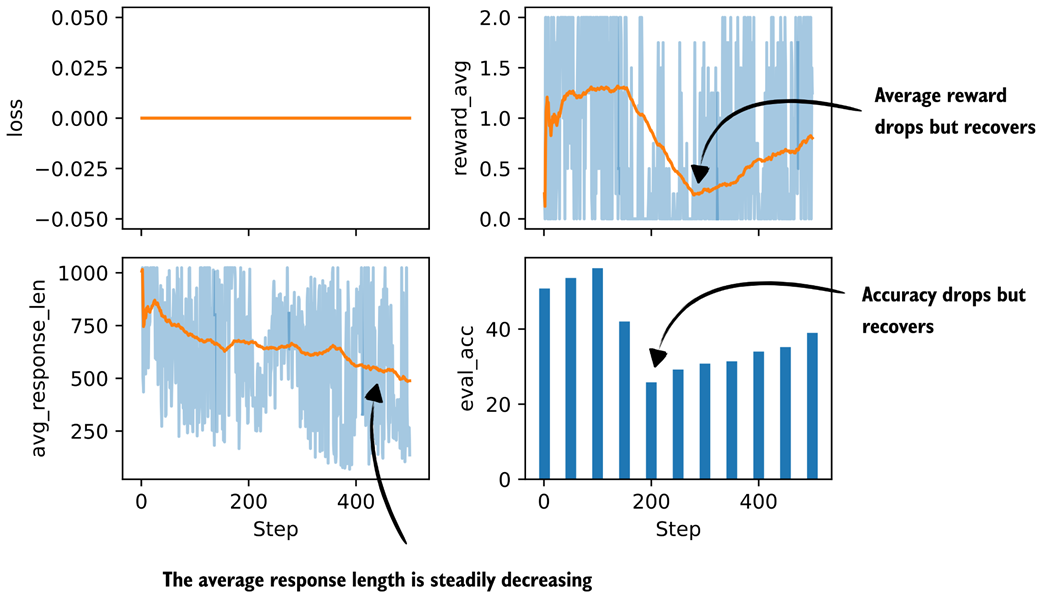 Figure B.1 Basic metrics from a GRPO training run with a conditional format reward.
The plots in Figure B.1 show that the evaluation accuracy and reward average take a big hit, but seem to recover.
Overall, despite this performance crash, it looks more stable than before, and the trend indicates that the performance would improve further if we trained longer.
plot_grpo_metrics(
    "7_6_plus_format_reward_conditional_metrics.csv",
    columns=["reward_avg", "format_reward_avg", "adv_std", "entropy_avg"],
)
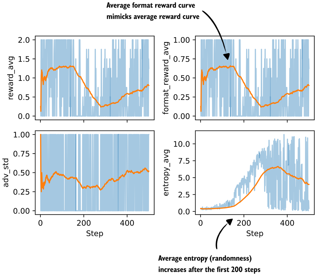 Figure B.2 Additional metrics from a GRPO training run with a conditional format reward.
In Figure B.2, we see the average format reward mimicking the average reward graph almost perfectly, which is a good sanity check that the conditional logic is working. Also, the average format reward shows how much of the total reward is coming from the format term on the subset of correct answers.
As we can see though, since the average format reward graph echoes the average reward one, it’s mainly a bonus (and it looks like it’s always awarded if the model is correct; this makes sense, because the trained reasoning model already knows how to use <think>...</think> tags correctly and we can see that it doesn’t unlearn this ability).
The entropy increase is still a bit troubling, though, and could hint towards training instabilities that could potentially be addressed by other means (like tighter clipping with smaller clip_eps).
B.7 Chapter 8
Exercise 8.1
To calculate the training and validation answer length statistics, you can add the following commands at the end of section 8.4.3, following the partitioning:
compute_length(train_examples)
# Prints
# Average: 1180 tokens
# Shortest: 236 tokens (index 5730)
# Longest: 2048 tokens (index 1319)
and
compute_length(val_examples)
# Prints
# Average: 1106 tokens
# Shortest: 310 tokens (index 12)
# Longest: 2048 tokens (index 15)
As we can see, the average token length (1180 versus 1106) is fairly similar, and the datasets should be relatively balanced.
As a bonus, we can also plot histograms to visualize the distributions:
import matplotlib.pyplot as plt

train_lengths = [len(ex["token_ids"]) for ex in train_examples]
val_lengths = [len(ex["token_ids"]) for ex in val_examples]

# Normalize counts because the validation split is much smaller
bins = range(0, max(train_lengths + val_lengths) + 64, 64)

fig, ax = plt.subplots(figsize=(7, 4))
ax.hist(train_lengths, bins=bins, density=True, alpha=0.6, label="Train")
ax.hist(val_lengths, bins=bins, density=True, alpha=0.6, label="Validation")
ax.set_xlabel("Token length")
ax.set_ylabel("Density")
ax.legend()
plt.tight_layout()
plt.show()
The resulting plot is shown in Figure B.3.
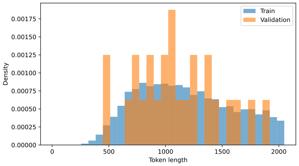 Figure B.3 Distribution of training and validation set lengths.
There are much fewer validation samples, which is why the validation histogram seems a bit jagged, but as we can see, it has a good distribution coverage.
Exercise 8.2
To replicate the run without <think></think> tokens in the script execution command:
uv run distill.py \
--data_path deepseek-r1-math-train.json \
--validation_size 25 \
--epochs 3 \
--lr 1e-5 \
--max_seq_len 2048 \
--grad_clip 1.0
Then, for the evaluation, we use the base instead of reasoning model:
uv run evaluate_math500.py \
--dataset_size 500 \
--which_model base \
--max_new_tokens 4096 \
--checkpoint_path \
run_11/checkpoints/distill/qwen3-0.6B-distill-step05746-epoch1.pth
The results are shown in table B.6.
Table B.6 MATH-500 task accuracy with and without think tokens
| Method | Epoch | Final val loss | MATH-500 Acc. | |
|---|---|---|---|---|
| 1 | Base Qwen3 0.6B (chapter 3) | - | - | 15.2% |
| 2 | Reasoning Qwen3 0.6B (chapter 3) | - | - | 48.2% |
| 3 | DeepSeek-R1 | 1 | 0.5436 (0.5404) | 31.8% (30.6%) |
| 4 | DeepSeek-R1 | 2 | 0.5349 (0.5339) | 31.8% (32.4%) |
| 5 | DeepSeek-R1 | 3 | 0.5343 (0.5306) | 30.2% (33.6%) |
| 6 | Qwen3 235B-A22B | 1 | 0.4043 (0.3130) | 44.8% (45.0%) |
| 7 | Qwen3 235B-A22B | 2 | 0.3963 (0.3087) | 39.4% (43.8%) |
| 8 | Qwen3 235B-A22B | 3 | 0.3948 (0.3078) | 39.8% (44.2%) |
In Table B.6, the new results (without think tokens) are shown first, with corresponding think-token results (from the main chapter) in parentheses.
Interestingly, the Qwen3 model has a lower validation loss when <think></think> tokens are omitted, but this doesn’t translate into better modeling performance.
As we can see, the omission of <think></think> makes the results slightly worse in almost all cases.