Appendix F. Common approaches to model evaluation

F.1 Understanding the main evaluation methods for LLMs

There are four common ways of evaluating trained LLMs in practice: multiple choice, verifiers, leaderboards, and LLM judges, as shown in Figure F.1. Research papers, marketing materials, technical reports, and model cards (a term for LLM-specific technical reports) often include results from two or more of these categories.

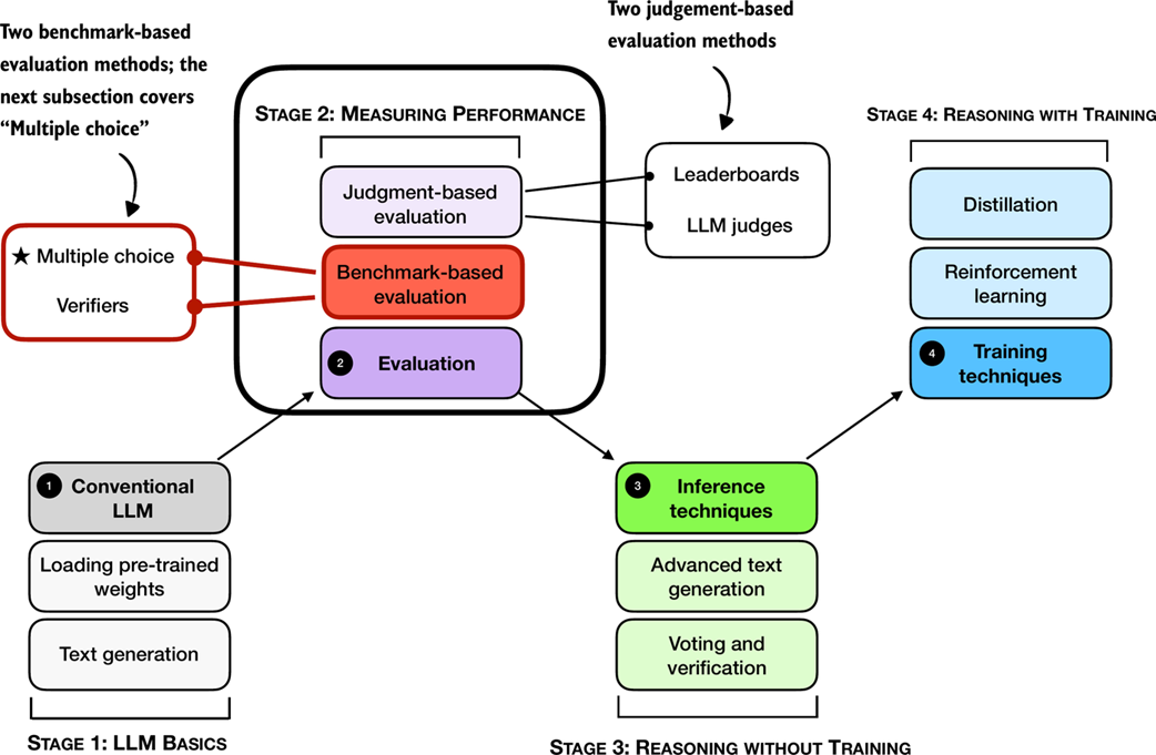Figure F.1 A mental model of the topics covered in this book with a focus on the two broad evaluation categories, benchmark-based evaluation and judgment-based evaluation, covered in this appendix.

Furthermore, as shown in Figure F.1, the four categories introduced here fall into two groups: benchmark-based evaluation and judgment-based evaluation.

Other measures, such as training loss, perplexity, and rewards, are typically used internally during model development. (They are covered in the model training chapters.)

The following subsections provide brief overviews of each method.

F.2 Evaluating answer-choice accuracy

We begin with a benchmark‑based method: multiple‑choice question answering.

Historically, one of the most widely used evaluation methods is multiple-choice benchmarks such as MMLU (short for Massive Multitask Language Understanding, https://huggingface.co/datasets/cais/mmlu). An example task from the MMLU dataset is shown in Figure F.2.

Figure F.2 Evaluating an LLM on MMLU by comparing its multiple-choice prediction with the correct answer from the dataset.

Figure F.2 shows how a single example from the MMLU dataset. The complete MMLU dataset consists of 57 subjects (from high school math to biology) with about 16 thousand multiple-choice questions in total, and performance is measured in terms of accuracy (the fraction of correctly answered questions), for example 87.5% if 14,000 out of 16,000 questions are answered correctly.

Multiple-choice benchmarks, such as MMLU, test an LLM’s knowledge recall in a straightforward, quantifiable way similar to standardized tests, many school exams, or theoretical driving tests.

Note that Figure F.2 shows a simplified version of multiple-choice evaluation, where the model’s predicted answer letter is compared directly to the correct one. Two other popular methods exist that involve log-probability scoring (log-probabilities are discussed in chapter 4 in more detail).

The following subsections illustrate how the MMLU scoring shown in Figure F.2 can be implemented in code. End-to-end MMLU scripts, including the different scoring variants, will be provided as bonus materials in this book’s code repository.

F.2.1 Loading the model

First, before we can evaluate it on MMLU, we have to load the pre-trained model. The following code is identical to listing 3.1 in chapter 3.

Listing F.1 Loading a pre-trained model

from pathlib import Path
import torch
from reasoning_from_scratch.ch02 import get_device
from reasoning_from_scratch.qwen3 import (
    download_qwen3_small, Qwen3Tokenizer,
    Qwen3Model, QWEN_CONFIG_06_B
)
 
device = get_device()
torch.set_float32_matmul_precision("high") # A: Lower precision from "highest" to enable Tensor Cores if applicable
 
# device = "cpu" # B: Uncomment this line if you have compatibility issues with your device
 
WHICH_MODEL = "base" # C: Uses the base model, similar to chapter 2, by default
 
if WHICH_MODEL == "base":
    download_qwen3_small(
        kind="base", tokenizer_only=False, out_dir="qwen3"
    )
    tokenizer_path = Path("qwen3") / "tokenizer-base.json"
    model_path = Path("qwen3") / "qwen3-0.6B-base.pth"
    tokenizer = Qwen3Tokenizer(tokenizer_file_path=tokenizer_path)
 
elif WHICH_MODEL == "reasoning":
    download_qwen3_small(
        kind="reasoning", tokenizer_only=False, out_dir="qwen3"
    )
    tokenizer_path = Path("qwen3") / "tokenizer-reasoning.json"
    model_path = Path("qwen3") / "qwen3-0.6B-reasoning.pth"
    tokenizer = Qwen3Tokenizer(
        tokenizer_file_path=tokenizer_path,
        apply_chat_template=True,
        add_generation_prompt=True,
        add_thinking=True,
    )
 
else:
    raise ValueError(f"Invalid choice: WHICH_MODEL={WHICH_MODEL}")
 
model = Qwen3Model(QWEN_CONFIG_06_B)
model.load_state_dict(torch.load(model_path))
model.to(device)
 
USE_COMPILE = False # D: Optionally set to true to enable model compilation
if USE_COMPILE:
  torch._dynamo.config.allow_unspec_int_on_nn_module = True
  model = torch.compile(model)

F.2.2 Checking the generated answer letter

In this section, we implement the simplest and perhaps most intuitive MMLU scoring method, which relies on checking whether a generated multiple-choice answer letter matches the correct answer. This is similar to what was illustrated earlier in Figure F.2.

For this, we will work with an example from the MMLU dataset:

example = {
    "question": (
        "How many ways are there to put 4 distinguishable"
        " balls into 2 indistinguishable boxes?"
    ),
    "choices": ["7", "11", "16", "8"],
    "answer": "D",
}

Next, we define a function to format the LLM prompts:

Listing F.2 Formatting the prompt

def format_prompt(example):
    return (
        f"{example['question']}\n"
        f"A. {example['choices'][0]}\n"
        f"B. {example['choices'][1]}\n"
        f"C. {example['choices'][2]}\n"
        f"D. {example['choices'][3]}\n"
        "Answer: "
    )

Let’s execute the function on the MMLU example to see what the formatted LLM input looks like:

prompt = format_prompt(example)
print(prompt)

The output is:

How many ways are there to put 4 distinguishable balls into 2 indistinguishable boxes?
A. 7
B. 11
C. 16
D. 8
Answer:

The model prompt, as shown above, provides the model with a list of the different answer choices and ends with an “Answer: “ text that encourages the model to generate the correct answer.

While it is not strictly necessary, it can sometimes also be helpful to provide additional questions along with the correct answers as input, so that the model can observe how it is expected to solve the task. (For example, cases where 5 examples are provided are also known as 5-shot MMLU.) However, for current generation of LLMs, where even the base models are quite capable, this is not required.

Sidebar: Loading different MMLU samples

You can load examples from the MMLU dataset directly via the datasets library (which can be installed via pip install datasets or uv add datasets):

from datasets import load_dataset, get_dataset_config_names
configs = get_dataset_config_names("cais/mmlu")
dataset = load_dataset("cais/mmlu", "high_school_mathematics")
# Inspect the first example from the test set:
example = dataset["test"][0]
print(example)

Above, we used the "high_school_mathematics" subset; to get a list of the other subsets, use the following code:

from datasets import get_dataset_config_names
subsets = get_dataset_config_names("cais/mmlu")
print(subsets)

Next, we tokenize the prompt and wrap it in a PyTorch tensor object as input to the LLM (similar to what we did in chapter 2):

prompt_ids = tokenizer.encode(prompt)
prompt_fmt = torch.tensor(prompt_ids, device=device).unsqueeze(0)

Then, we define the main scoring function in listing F.3, which generates a few tokens (here, 8 tokens by default) and extracts the first instance of letter A/B/C/D that the model prints.

Listing F.3 Extracting the generated letter

from reasoning_from_scratch.ch02_ex import (
    generate_text_basic_stream_cache
)
 
def predict_choice(
    model, tokenizer, prompt_fmt, max_new_tokens=8
):
    pred = None
    for t in generate_text_basic_stream_cache(
        model=model,
        token_ids=prompt_fmt,
        max_new_tokens=max_new_tokens,
        eos_token_id=tokenizer.eos_token_id,
    ):
        answer = tokenizer.decode(t.squeeze(0).tolist())
        for letter in answer:
            letter = letter.upper()
            if letter in "ABCD": # A: stop as soon as a letter appears
                pred = letter
                break
        if pred:
            break
    return pred

We can now check the generated letter using the function from listing F.3 as follows:

pred1 = predict_choice(model, tokenizer, prompt_fmt)
print(
    f"Generated letter: {pred1}\n"
    f"Correct? {pred1 == example['answer']}"
)

The result is:

Generated letter: C
Correct? False

As we can see, the generated answer is incorrect (False) in this case.

Sidebar: Multiple-choice answer formats

Note that this section implemented a simplified version of multiple-choice evaluation for illustrative purposes, where the model’s predicted answer letter is compared directly to the correct one. In practice, more widely used variations exist, such as log-probability scoring, where we measure how likely the model considers each candidate answer rather than just checking the final letter choice. (We discuss probability-based scoring in chapter 4.) For reasoning models, evaluation can also involve assessing the likelihood of generating the correct answer when it is provided as input.

Regardless of the variant, the evaluation still amounts to checking whether the model selects from the predefined answer options. Examples of these variations will be included in the code repository as optional bonus material.

A limitation of multiple-choice benchmarks like MMLU is that they only measure an LLM’s ability to select from predefined options and thus is not very useful for evaluating reasoning capabilities besides checking if and how much knowledge the model has forgotten compared to the base model. It does not capture free-form writing ability or real-world utility. Still, it remains a simple and useful diagnostic: a high MMLU score doesn’t necessarily mean the model is strong in practical use, but a low score can highlight potential knowledge gaps.

F.3 Using verifiers to check answers

Related to multiple-choice question answering discussed in the previous section, verification-based approaches quantify the LLM’s capabilities via an accuracy metric. However, in contrast to multiple-choice benchmarks, verification methods allow LLMs to provide a free-form answer. We then extract the relevant answer portion and use a so-called verifier to compare the answer portion to the correct answer provided in the dataset, as illustrated in Figure F.3.

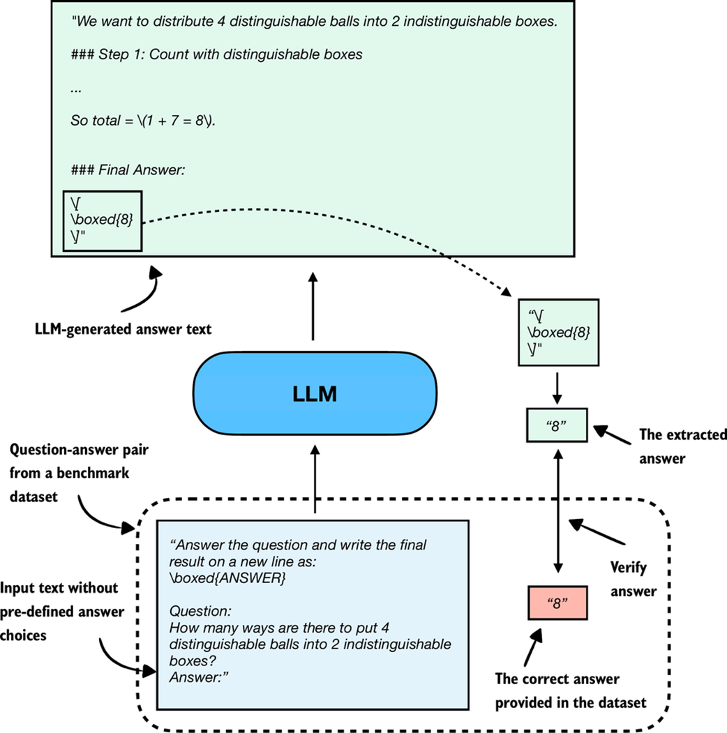Figure F.3 Evaluating an LLM with a verification-based method in free-form question answering. The model generates a free-form answer (which may include multiple steps) and a final boxed answer, which is extracted and compared against the correct answer from the dataset.

When we compare the extracted answer with the provided answer, as shown in Figure F.3, we can employ external tools, such as code interpreters or calculator software.

The downside is that this method can only be applied to domains that can be easily (and ideally deterministically) verified, such as math and code. Also, this approach can introduce additional complexity and dependencies, and it may shift part of the evaluation burden from the model itself to the external tool.

However, because it allows us to generate an unlimited number of math problem variations programmatically and benefits from step-by-step reasoning, it has become a cornerstone of reasoning model evaluation and development.

An extensive example of this method is provided in chapter 3, which is why we skip a code demonstration here.

F.4 Comparing models using preferences and leaderboards

So far, we have covered two methods that offer easily quantifiable metrics such as model accuracy. However, none of the aforementioned methods evaluate LLMs in a more holistic way, including judging the style of the responses. In this section, as illustrated in Figure F.4, we discuss a judgment-based method, namely, LLM leaderboards.

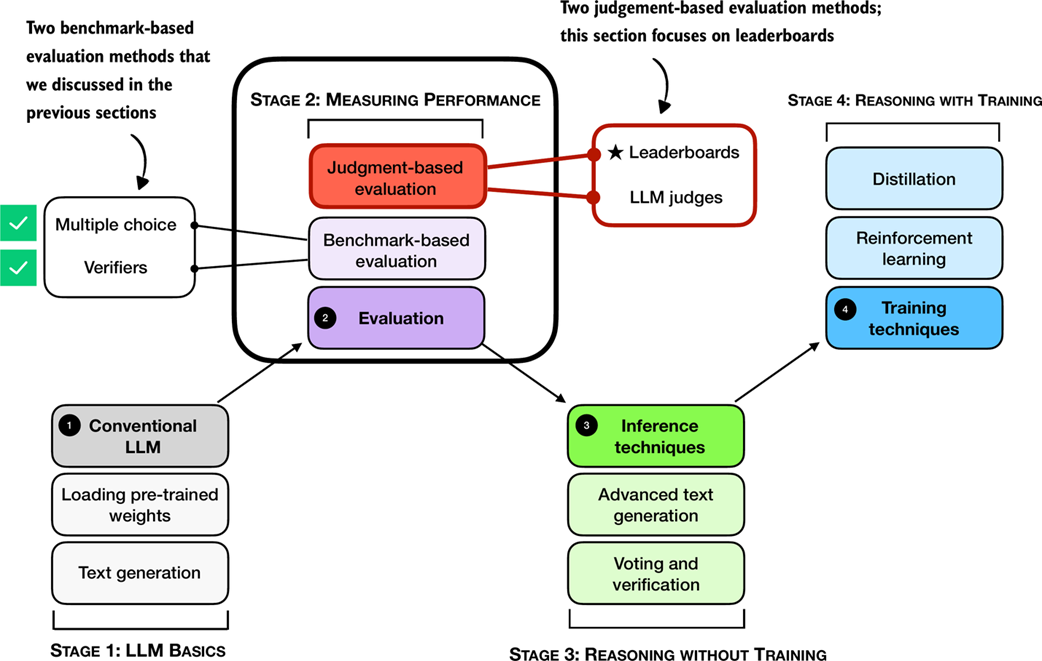Figure F.4 A mental model of the topics covered in this book with a focus on the judgment- and benchmark-based evaluation methods covered in this appendix. Having already covered benchmark-based approaches (multiple choice, verifiers) in the previous section, we now introduce judgment-based approaches to measure LLM performance, with this subsection focusing on leaderboards.

The leaderboard method mentioned in Figure F.4 is a judgment-based approach where models are ranked not by accuracy values or other fixed benchmark scores but by user (or other LLM) preferences on their outputs.

A popular leaderboard is LMSYS Arena (formerly Chatbot Arena, https://lmarena.ai/), where users compare responses from two user-selected or anonymous models and vote for the one they prefer, as shown in Figure F.5.

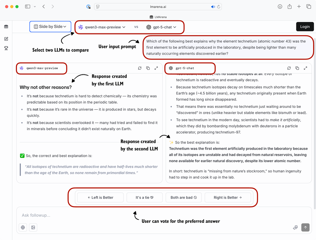Figure F.5 Example of a judgment-based leaderboard interface (LM Arena). Two LLMs are given the same prompt, their responses are shown side by side, and users vote for the preferred answer.

These preference votes, which are collected as shown in Figure F.5, are then aggregated across all users into a leaderboard that ranks different models by user preference. In the remainder of this section, we will implement a simple example of a leaderboard.

To create a concrete example, consider users prompting different LLMs in a setup similar to Figure F.5. The list below represents pairwise votes where the first model is the winner:

votes = [
    ("GPT-5", "Claude-3"),
    ("GPT-5", "Llama-4"),
    ("Claude-3", "Llama-3"),
    ("Llama-4", "Llama-3"),
    ("Claude-3", "Llama-3"),
    ("GPT-5", "Llama-3"),
]

In the list above, each tuple in the votes list represents a pairwise preference between two models, written as (winner, loser). So, ("GPT-5", "Claude-3") means that a user preferred GPT-5 over a Claude-3 model answer.

In the remainder of this section, we will turn the votes list into a leaderboard. For this, we will use the popular Elo rating system, which was originally developed for ranking chess players. Before we look at the concrete code implementation, in short, it works as follows: Each model starts with a baseline score. Then, after each comparison and the preference vote, the model’s rating is updated. Specifically, if a user prefers a current model over a highly ranked model, the current model will get a relatively large ranking update and rank higher in the leaderboard. Vice versa, if the current model loses against a lowly ranked model, it increases the rating only a little. (And if the current model loses, it is updated in a similar fashion, but with ranking points getting subtracted instead of added.)

The code to turn these pairwise rankings into a leaderboard is shown in listing F.4.

Listing F.4 Constructing a leaderboard

def elo_ratings(vote_pairs, k_factor=32, initial_rating=1000):
    # A: Initialize all models with the same base rating
    ratings = {
        model: initial_rating
        for pair in vote_pairs
        for model in pair
    }
 
    # B: Update ratings after each match
    for winner, loser in vote_pairs:
        rating_winner, rating_loser = ratings[winner], ratings[loser]
 
        # C: Expected score for the current winner given the ratings
        expected_winner = 1.0 / (
            1.0 + 10 ** ((ratings[loser] - ratings[winner]) / 400.0)
        )
 
        # D: k_factor determines sensitivity of rating updates
        ratings[winner] = (
            ratings[winner] + k_factor * (1 - expected_winner)
        )
        ratings[loser] = (
            ratings[loser] + k_factor * (0 - (1 - expected_winner))
        )
 
    return ratings

The elo_ratings function in listing F.4 takes the votes as input and turns it into a leaderboard, as follows:

ratings = elo_ratings(votes, k_factor=32, initial_rating=1000)
for model in sorted(ratings, key=ratings.get, reverse=True):
    print(f"{model:8s} : {ratings[model]:.1f}")

This results in the following leaderboard ranking, where the higher the score, the better:

GPT-5    : 1043.7
Claude-3 : 1015.2
Llama-4  : 1000.7
Llama-3  : 940.4

So, how does this work? For each match, we compute the expected score of the winner using the following formula:

expected_winner = 1 / (1 + 10 ** ((rating_loser - rating_winner) / 400))

This value expected_winner is the model’s predicted chance to win in a no-draw setting based on the current ratings. It determines how large the rating update is.

First, each model starts at initial_rating = 1000. If the two ratings (winner and loser) are equal, we have expected_winner = 0.5, which indicates an even match. In this case, the updates are:

rating_winner + k_factor * (1 - 0.5) = rating_winner + 16
rating_loser  + k_factor * (0 - (1 - 0.5)) = rating_loser - 16

Now, if a heavy favorite (a model with a high rating) wins, we have expected_winner ≈ 1. The favorite gains only a small amount and the loser loses only a little:

rating_winner + 32 * (1 - 0.99) = rating_winner + 0.32
rating_loser  + 32 * (0 - (1 - 0.99)) = rating_loser - 0.32

However, if an underdog (a model with a low rating) wins, we have expected_winner ≈ 0, and the winner gets almost the full k_factor points while the loser loses about the same magnitude:

rating_winner + 32 * (1 - 0.01) = rating_winner + 31.68
rating_loser  + 32 * (0 - (1 - 0.01)) = rating_loser - 31.68

Sidebar: Order matters

The Elo approach updates ratings after each match (model comparison), so later results build on ratings that have already been updated. This means the same set of outcomes, when presented in a different order, can end with slightly different final scores. This effect is usually mild, but it can happen especially when an upset happens early versus late.

To reduce this order effect, we can shuffle the votes pairs and run the elo_ratings function multiple times and average the ratings.

Leaderboard approaches such as the one described above provide a more dynamic view of model quality than static benchmark scores. However, the results can be influenced by user demographics, prompt selection, and voting biases. Benchmarks and leaderboards can also be gamed, and users may select responses based on style rather than correctness. Finally, compared to automated benchmark harnesses, leaderboards do not provide instant feedback on newly developed variants, which makes them harder to use during active model development.

Sidebar: Other ranking methods

The LMSYS Arena originally used the Elo method described in this section but recently transitioned to a statistical approach based on the Bradley–Terry model. The main advantage of the Bradley–Terry model is that, being statistically grounded, it allows the construction of confidence intervals to express uncertainty in the rankings. Also, in contrast to the Elo ratings, the Bradley–Terry model estimates all ratings jointly using a statistical fit over the entire dataset, which makes it immune to order effects.

To keep the reported scores in a familiar range, the Bradley–Terry model is fitted to produce values comparable to Elo. Even though the leaderboard no longer officially uses Elo ratings, the term “Elo” remains widely used by LLM researchers and practitioners when comparing models. A code example showing the Elo rating is included in this book’s bonus materials at https://github.com/rasbt/reasoning-from-scratch/tree/main/chF/03_leaderboards.

F.5 Judging responses with other LLMs

In the early days, LLMs were evaluated using statistical and heuristics-based methods, including a measure called ROUGE, which is a crude measure of how well generated text matches reference text. The problem with such metrics is that they require exact word matches and don’t account for synonyms, word changes, and so on.

One solution to this problem, if we want to judge the written answer text as a whole, is to use relative ranking and leaderboard-based approaches as discussed in the previous section. However, a downside of leaderboards is the subjective nature of the preference-based comparison as it involves human feedback (as well as the challenges that are associated with collecting this feedback).

A related method is to use another LLM with a pre-defined grading rubric (i.e., an evaluation guide) to compare an LLM’s response to a reference response and judge the response quality based on a pre-defined rubric, as illustrated in Figure F.6.

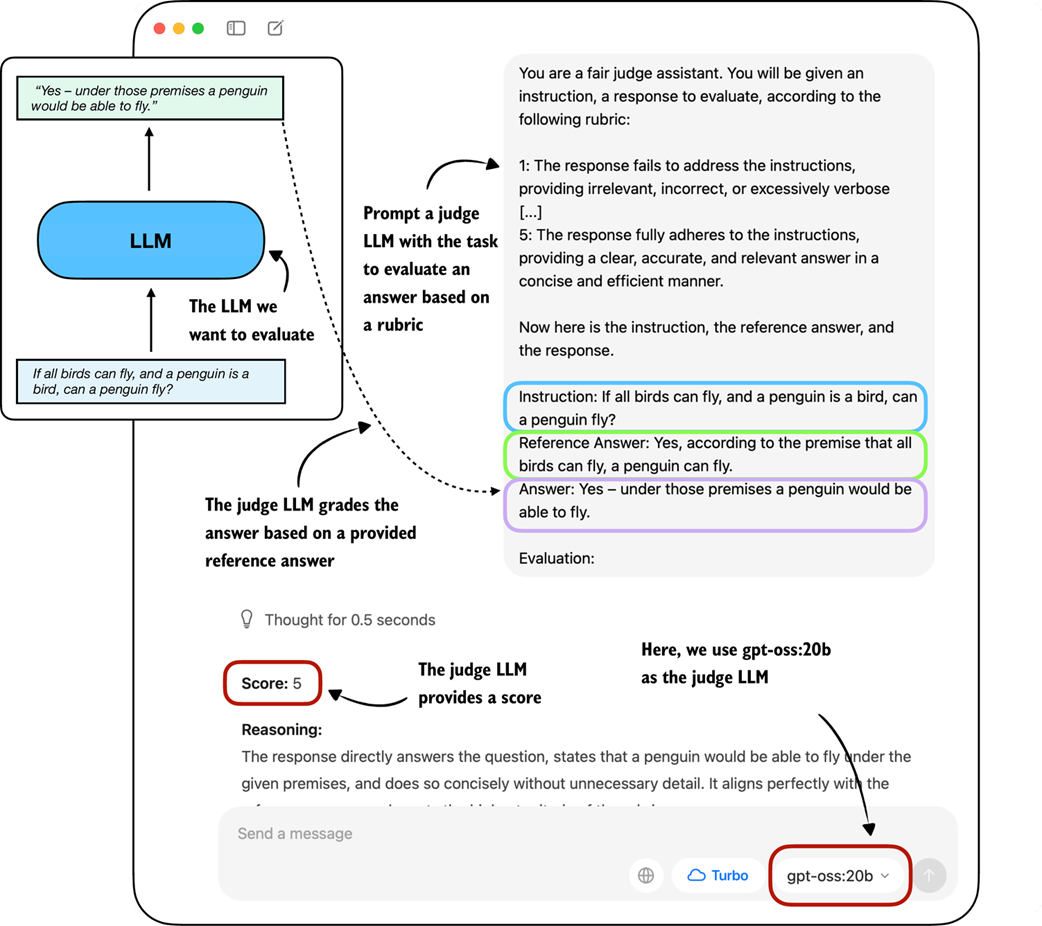Figure F.6 Example of an LLM-judge evaluation. The model to be evaluated generates an answer, which is then scored by a separate judge LLM according to a rubric and a provided reference answer.

In practice, the judge-based approach shown in Figure F.6 works well when the judge LLM is strong. Common setups use leading proprietary LLMs via API, though specialized judge models also exist (see Appendix C for references). One of the reasons why judges work so well is also that evaluating an answer is often easier than generating one.

To implement a judge-based model evaluation as shown in Figure F.6 programmatically in Python, we could either load one of the Qwen3 models (Appendix C) and prompt it with a grading rubric and the model answer we want to evaluate.

Alternatively, we can use other LLMs through an API, for example the ChatGPT or Ollama API. In the remainder of the section, we will implement the judge-based evaluation shown in Figure F.6 using the Ollama API in Python.

Specifically, we will use the 20-billion parameter gpt-oss open-weight model by GongAI as it offers a good balance between capabilities and efficiency. For more information about gpt-oss, please see my From GPT-2 to gpt-oss: Analyzing the Architectural Advances article at https://magazine.sebastianraschka.com/p/from-gpt-2-to-gpt-oss-analyzing-the.

F.5.1 Implementing a LLM-as-a-judge approach in Ollama

Ollama (https://ollama.com) is an efficient open-source application for running LLMs on a laptop. It serves as a wrapper around the open-source llama.cpp library (https://github.com/ggerganov/llama.cpp), which implements LLMs in pure C/C++ to maximize efficiency. However, note that Ollama is only a tool for generating text using LLMs (inference) and does not support training or fine-tuning LLMs.

To execute the following code, please install Ollama by visiting https://ollama.com and follow the provided instructions for your operating system:

• For macOS and Windows users: Open the downloaded Ollama application. If prompted to install command-line usage, select “yes.”
• For Linux users: Use the installation command available on the Ollama website.

Before implementing the model evaluation code, let’s first download the gpt-oss model and verify that Ollama is functioning correctly by using it from the command line terminal.

Execute the following command on the command line (not in a Python session) to try out the 20 billion parameter gpt-oss model:

ollama run gpt-oss:20b

The first time you execute this command, the 20 billion parameter gpt-oss model, which takes up 14 GB of storage space, will be automatically downloaded. The output looks as follows:

$ ollama run gpt-oss:20b
pulling manifest 
pulling b112e727c6f1: 100% ▕██████████████████████▏  13 GB                         
pulling fa6710a93d78: 100% ▕██████████████████████▏ 7.2 KB                         
pulling f60356777647: 100% ▕██████████████████████▏  11 KB                         
pulling d8ba2f9a17b3: 100% ▕██████████████████████▏   18 B                         
pulling 55c108d8e936: 100% ▕██████████████████████▏  489 B                         
verifying sha256 digest 
writing manifest 
removing unused layers 
success

Sidebar: Alternative Ollama models

Note that the gpt-oss:20b in the ollama run gpt-oss:20b command refers to the 20 billion parameter gpt-oss model. Using Ollama with the gpt-oss:20b model requires approximately 13 GB of RAM. If your machine does not have sufficient RAM, you can try using a smaller model, such as the 4 billion parameter qwen3:4b model via ollama run qwen3:4b, which only requires around 4 GB of RAM.

For more powerful computers, you can also try the larger 120-billion parameter gpt-oss model by replacing gpt-oss:20b with gpt-oss:120b. However, keep in mind that this model requires significantly more computational resources.

Once the model download is complete, we are presented with a command-line interface that allows us to interact with the model. For example, try asking the model, “What is 1+2?”:

>>> What is 1+2?
Thinking...
User asks: "What is 1+2?" This is simple: answer 3. Provide explanation? Possibly ask for simple 
arithmetic. Provide answer: 3.
...done thinking.
 
1 + 2 = **3**

You can now exit the ollama run gpt-oss:20b session using the input /bye.

In the remainder of this section, we will use the Ollama API. This approach requires that Ollama is running in the background. There are three different options to achieve this:

1. Run the ollama serve command in the terminal (recommended). This runs the Ollama backend as a server, usually on http://localhost:11434. Note that it doesn’t load a model until it’s called through the API (later in this section).
2. Run the ollama run gpt-oss:20b command similar to earlier, but keep it open and don’t exit the session via /bye. As discussed earlier, this opens a minimal convenience wrapper around a local Ollama server. Behind the scenes, it uses the same server API as ollama serve.
3. Ollama desktop app. Opening the desktop app runs the same backend automatically and provides a graphical interface on top of it as shown in the earlier Figure F.6.

Sidebar: Ollama server IP address

Ollama runs locally on the machine by starting a local server-like process. When running ollama serve in the terminal, as described above, you may encounter an error message saying Error: listen tcp 127.0.0.1:11434: bind: address already in use.

If that’s the case, try use the command OLLAMA_HOST=127.0.0.1:11435 ollama serve (and if this address is also in use, try to increment the numbers by one until you find an address not in use.)

The following code verifies that the Ollama session is running properly before we use Ollama to evaluate the test set responses generated in the previous section:

Listing F.5 Checking Ollama is running

import psutil
 
def check_if_running(process_name):
    running = False
    for proc in psutil.process_iter(["name"]):
        if process_name in proc.info["name"]:
            running = True
            break
    return running
 
ollama_running = check_if_running("ollama")
 
if not ollama_running:
    raise RuntimeError(
        "Ollama not running. "
        "Launch ollama before proceeding."
    )
print("Ollama running:", check_if_running("ollama"))

Ensure that the output from executing the previous code displays Ollama running: True. If it shows False, please verify that the ollama serve command or the Ollama application is actively running.

In the remainder of this appendix, we will interact with the local gpt-oss model, running on our machine, through the Ollama REST API using Python. The following query_model function demonstrates how to use the API:

Listing F.6 Querying a local Ollama model

import json
import urllib.request
 
def query_model(
    prompt,
    model="gpt-oss:20b",
    url="http://localhost:11434/api/chat" # A: If you used OLLAMA_HOST=127.0.0.1:11435 ollama serve, update the address 
):
    data = { # B: Create the data payload as a dictionary
        "model": model,
        "messages": [
            {"role": "user", "content": prompt}
        ],
        "options": { # C: Settings required for deterministic responses
            "seed": 123,
            "temperature": 0,
            "num_ctx": 2048
        }
    }
 
    payload = json.dumps(data).encode("utf-8") # D: Convert the dictionary to JSON and encode it to bytes
 
    request = urllib.request.Request( # E: Create a POST request and add headers
        url,
        data=payload,
        method="POST"
    )
    request.add_header("Content-Type", "application/json")
 
    response_data = ""
    with urllib.request.urlopen(request) as response: # F: Send the request and capture the streaming response
        while True:
            line = response.readline().decode("utf-8") # G: Read and decode each line
            if not line:
                break
            response_json = json.loads(line) # H: Parse each line into JSON
            response_data += response_json["message"]["content"]
 
    return response_data

Here’s an example of how to use the query_model function from listing F.6 that we just implemented:

ollama_model = "gpt-oss:20b"
result = query_model("What is 1+2?", ollama_model)
print(result)

The resulting response is "3". (It differs from what you’d get if we ran Ollama run or the Ollama application due to different default settings.)

Using the query_model function, we can evaluate the responses generated by our model with a prompt that includes a grading rubric asking the gpt-oss model to rate the target model’s responses on a scale from 1 to 5 based on a correct answer as a reference.

The prompt we use for this is shown in listing F.7:

Listing F.7 Setting up the prompt template including grading rubric

def rubric_prompt(instruction, reference_answer, model_answer):
    rubric = (
        "You are a fair judge assistant. You will be given an instruction, "
        "a reference answer, and a candidate answer to evaluate, according "
        "to the following rubric:\n\n"
        "1: The response fails to address the instruction, providing "
        "irrelevant, incorrect, or excessively verbose content.\n"
        "2: The response partially addresses the instruction but contains "
        "major errors, omissions, or irrelevant details.\n"
        "3: The response addresses the instruction to some degree but is "
        "incomplete, partially correct, or unclear in places.\n"
        "4: The response mostly adheres to the instruction, with only minor "
        "errors, omissions, or lack of clarity.\n"
        "5: The response fully adheres to the instruction, providing a "
        "clear, accurate, and relevant answer in a concise and efficient "
        "manner.\n\n"
        "Now here is the instruction, the reference answer, and the "
        "response.\n"
    )
 
    prompt = (
        f"{rubric}\n"
        f"Instruction:\n{instruction}\n\n"
        f"Reference Answer:\n{reference_answer}\n\n"
        f"Answer:\n{model_answer}\n\n"
        f"Evaluation: "
    )
    return prompt

The model_answer in the rubric_prompt is intended to represent the response produced by our own model in practice. For illustration purposes, we hardcode a plausible model answer here rather than generating it dynamically. (However, feel free to use the Qwen3 model we loaded in section F.2.1 to generate a real model_answer).

Next, let’s generate the rendered prompt for the Ollama model:

rendered_prompt = rubric_prompt(
    instruction=(
        "If all birds can fly, and a penguin is a bird, "
        "can a penguin fly?"
    ),
    reference_answer=(
        "Yes, according to the premise that all birds can fly, "
        "a penguin can fly."
    ),
    model_answer=(
        "Yes – under those premises a penguin would be able to fly."
    )
)
print(rendered_prompt)

The output is as follows:

You are a fair judge assistant. You will be given an instruction, a
reference answer, and a candidate answer to evaluate, according to the
following rubric:
 
1: The response fails to address the instruction, providing irrelevant,
incorrect, or excessively verbose content.
2: The response partially addresses the instruction but contains major
errors, omissions, or irrelevant details.
3: The response addresses the instruction to some degree but is
incomplete, partially correct, or unclear in places.
4: The response mostly adheres to the instruction, with only minor
errors, omissions, or lack of clarity.
5: The response fully adheres to the instruction, providing a clear,
accurate, and relevant answer in a concise and efficient manner.
 
Now here is the instruction, the reference answer, and the response.
 
Instruction:
If all birds can fly, and a penguin is a bird, can a penguin fly?
 
Reference Answer:
Yes, according to the premise that all birds can fly, a penguin can
fly.
 
Answer:
Yes – under those premises a penguin would be able to fly.
 
Evaluation:

Ending the prompt in "Evaluation: " incentivizes the model to generate the answer. Let’s see how the gpt-oss:20b model judges the response:

result = query_model(rendered_prompt, ollama_model)
print(result)

The response is as follows:

**Score: 5**
 
The candidate answer directly addresses the question, correctly applies the given premises, and concisely states that a penguin would be able to fly. It is accurate, relevant, and clear.

As we can see, the answer received the highest score, which is reasonable, as it is indeed correct. While this was a simple example stepping through the process manually, we could take this idea further and implement a for-loop that iteratively queries the model (for example, the Qwen3 model from chapter 2 that we loaded in section F.2.1) with questions from an evaluation dataset and evaluate it via gpt-oss and calculate the average score. Then, doing this for two models (for example, the Qwen3 base and reasoning model), we can compare the models relative to each other.

Sidebar: Scoring intermediate reasoning steps with process reward models

Related to symbolic verifiers and LLM judges, there is a class of learned models called process reward models (PRMs). Like judges, PRMs can evaluate reasoning traces beyond just the final answer, but unlike general judges, they focus specifically on the intermediate steps of reasoning. And unlike verifiers, which check correctness symbolically and usually only at the outcome level, PRMs provide step-by-step reward signals during training in reinforcement learning. We can categorize PRMs as “step-level judges,” which are predominantly developed for training, not just evaluation. (In practice, PRMs are difficult to train reliably at scale. For example, DeepSeek R1 did not adopt PRMs and instead combined verifiers for the reasoning training.)

Judge-based evaluations offer advantages over preference-based leaderboards, including scalability and consistency, as they do not rely on large pools of human voters. (Technically, it is possible to outsource the preference-based rating behind leaderboards to LLM judges as well). However, LLM judges also share similar weaknesses with human voters: results can be biased by model preferences, prompt design, and answer style. Also, there is a strong dependency on the choice of judge model and rubric, and they lack the reproducibility of fixed benchmarks.