Inference-time Scaling via Self-Refinement
Chapter 5: Inference-time scaling via self-refinement
This chapter covers
- Scoring LLM answers with a simple rule-based scorer
- Computing an LLM’s own confidence in its answers
- Coding a self-refinement loop where the LLM iteratively improves its answers
The previous chapter introduced the concept of inference-time scaling (inference scaling for short), which improves the model response accuracy without further training the model. In particular, the focus of the previous chapter was on self-consistency, where the model generates multiple answers, and the final answer is chosen by majority vote.
As outlined in figure 5.1, this chapter moves beyond simple majority voting for inference scaling and covers another popular and useful inference-scaling technique, self-refinement. Instead of generating multiple answers to choose from, self-refinement focuses on iteratively refining a single answer to correct potential mistakes.
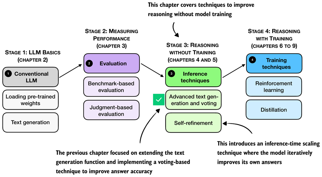 Figure 5.1 A mental model of the topics covered in this book. This chapter continues stage 3 and focuses on inference-time techniques for improving reasoning without additional training. This chapter introduces self-refinement, where the model iteratively critiques and improves its own answers.
5.1 Scoring and iteratively improving model responses
As discussed in the previous chapter, inference scaling provides a way to trade additional compute for better accuracy. We also covered two inference scaling techniques, chain-of-thought prompting and self-consistency.
Chain-of-thought prompting, as illustrated in figure 5.2, modifies the prompt, for example, by adding the phrase “Explain step by step.”, which can trigger the model to write longer explanations which can in turn result in better answer accuracy. This method is particularly useful for base models that don’t naturally provide reasoning-like explanations. However, models trained as reasoning models usually don’t benefit from this type of inference scaling, since they already explain their answers.
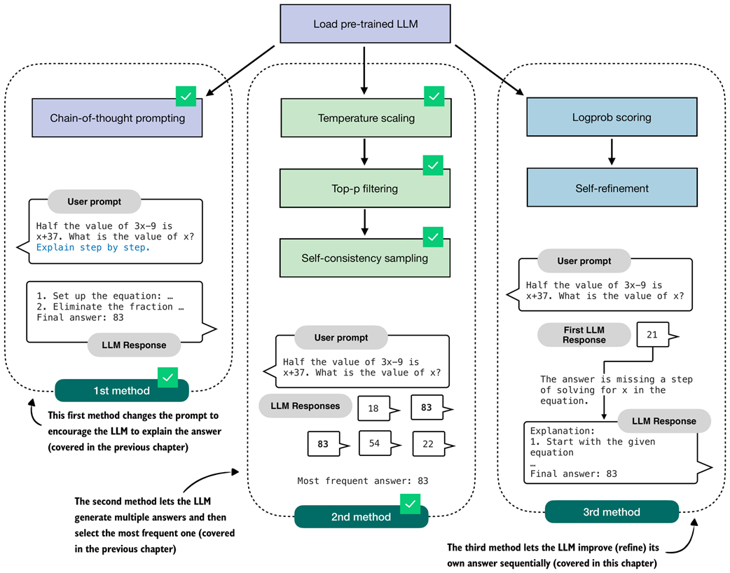 Figure 5.2 Overview of three inference-time methods to improve reasoning covered in this book. The first two methods were covered in the previous chapter. This chapter covers the third method, self-refinement, where the model iteratively improves its own answers.
Self-consistency, the second method shown in figure 5.2, lets the model produce several answers in parallel. We then pick the final answer by taking a simple majority vote over these candidates.
Even though self-consistency is quite simple, it often yields large gains in answer accuracy, which is why it has become a common choice in LLM applications where accuracy is a higher priority than latency. Recent examples include DeepSeekMath-7B and Google’s Gemini 1.5 Long Context mode (see appendix C for references).
However, one downside of self-consistency is that majority voting requires short answers that can be compared.
In this chapter, we implement a more versatile technique, self-refinement, in which the LLM learns to improve its own answers iteratively (method 3 in figure 5.2).
But before we implement the self-refinement technique, we will first implement scoring functions that we will use to compare and rank different answers, as outlined in figure 5.3.
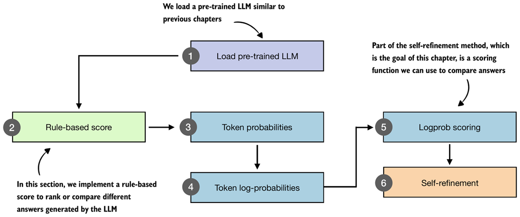 Figure 5.3 Overview of the components introduced in this chapter. We build a simple rule-based score, compute token probabilities and log-probabilities, and then use these scores as part of a self-refinement method where the model iteratively improves its own answers.
After loading the pre-trained LLM, as in previous chapters (step 1 in figure 5.3), we will start this chapter with a simple rule-based scoring function to illustrate the concept of scoring (step 2). Then, we will go over the concepts of token probabilities (step 3) and token log-probabilities (step 4), which we will need to implement the logprob scoring method (step 5) for our self-refinement loop (step 6).
We will primarily use the logprob scoring function (step 5 in figure 5.3) to track the progress within the self-refinement loop. However, these scoring functions can also be used to break ties in self-consistency or select the best response instead of relying on a majority vote.
The chapter overview in figure 5.3, leading up to self-refinement, looks relatively short and straightforward. However, the topics of token probability and log-probability are somewhat complex and will also be relevant in the next chapter, where we implement reinforcement learning methods to train the LLM. So, this chapter will spend a significant portion on explaining the concept of log-probability scoring.
5.2 Loading a pre-trained model
As in the previous chapter, we begin by loading the model used throughout this chapter.
Listing 5.1 Load tokenizer and base model
import torch
from reasoning_from_scratch.ch02 import get_device
from reasoning_from_scratch.ch03 import (
     load_model_and_tokenizer
)

device = get_device()
device = torch.device("cpu") # Delete this line to run the code on a GPU (if supported by your machine)

model, tokenizer = load_model_and_tokenizer(
    which_model="base",
    device=device,
    use_compile=False
)
As in previous chapters, the code in listing 5.1 loads the model and tokenizer used throughout this chapter.
Note that the code above runs on the CPU by default to ensure results that are generally more consistent with those shown in this chapter. While small numerical differences can still occur on the CPU depending on the operating system and machine, these differences are typically smaller and more predictable than those observed across different accelerator backends.
Later sections (sections 5.4 and 5.5) use computations involving very small numbers with many digits after the decimal point, which are more sensitive to device choice and low-level implementation details. This is not an issue in practice, but such mismatches can be confusing on a first read-through. For that reason, I recommend starting with the CPU device and considering MPS or CUDA devices later.
Next, to ensure that the model is loaded correctly, let’s use it together with the temperature and top-p sampler code from the previous chapter on a MATH-500 prompt:
Listing 5.2 Generating text with temperature scaling and top-p sampling
from reasoning_from_scratch.ch03 import render_prompt
from reasoning_from_scratch.ch04 import (
    generate_text_stream_concat_flex,
    generate_text_top_p_stream_cache
)

raw_prompt = (
    "Half the value of $3x-9$ is $x+37$. "
    "What is the value of $x$?"
)
prompt = render_prompt(raw_prompt)
prompt_cot = prompt + "\n\nExplain step by step."

torch.manual_seed(0)
response_1 = generate_text_stream_concat_flex(
    model, tokenizer, prompt_cot, device,
    max_new_tokens=2048, verbose=True,
    generate_func=generate_text_top_p_stream_cache,
    temperature=0.9,
    top_p=0.9
)
The model produces the following response:
The problem states that half the value of 3x−9 is equal to x+37. We need to find the value of \(x\).

### Step 2: Translate the problem into an equation
...

### Final Answer

\[
\boxed{83}
\]
Because we are using temperature scaling and top-p sampling, changing the random seed produces a different response:
torch.manual_seed(3)
response_2 = generate_text_stream_concat_flex(
    model, tokenizer, prompt_cot, device,
    max_new_tokens=2048, verbose=True,
    generate_func=generate_text_top_p_stream_cache,
    temperature=0.9,
    top_p=0.9,
)
This time, the model responds as follows:
We start with the given equation:
\[
\frac{1}{2} \times (3x - 9) = x + 37
\]
...
Final Answer:
\[
\boxed{83}
\]
In both cases, the model produces the correct final answer (83). However, the second response is much shorter, which we can confirm by printing the number of characters or tokens in each response:
print("Response 1 characters:", len(response_1))
print("Response 1 tokens:", len(tokenizer.encode(response_1)))
print("\nResponse 2 characters:", len(response_2))
print("Response 2 tokens:", len(tokenizer.encode(response_2)))
The result is:
Response 1 characters: 1419
Response 1 tokens: 534

Response 2 characters: 533
Response 2 tokens: 231
A shorter response is not necessarily better. If two responses reach the same correct answer, judging which one is better is not straightforward. It often depends on human preferences regarding clarity, usefulness, and the partial correctness of the intermediate steps.
Scoring intermediate steps of a response remains an active research area (see appendix C), and methods such as process reward models, which evaluate the reasoning itself, do not always yield better outputs in practice.
If the qualitative value of two responses is comparable, one thing is certain: shorter responses are cheaper because they require generating fewer tokens and are therefore preferred.
5.3 Scoring LLM responses with a rule-based score
In the previous section, the LLM generated two correct responses. In this section, we develop a simple rule-based scoring function to compare them (figure 5.4).
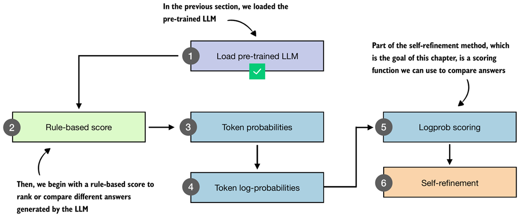 Figure 5.4 This section implements a rule-based scorer to rank different answers generated by the pre-trained LLM.
The rule-based scoring function assigns a score to each of two LLM responses (figure 5.5), which allows us to rank them and select the better one. Here, “better” refers to format and brevity, not correctness.
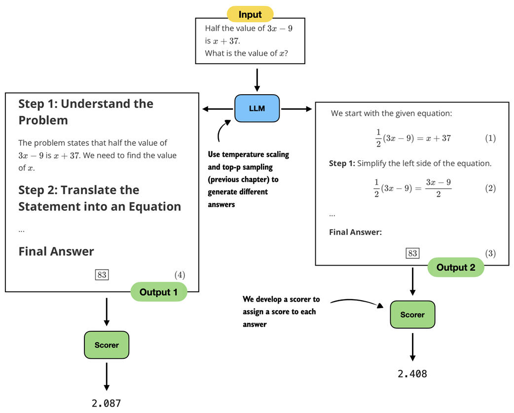 Figure 5.5 Two generated responses reach the same correct answer but differ in their explanations. A scorer evaluates the responses and assigns a score to each response.
There are several ways to implement a scoring function (scorer) for evaluating responses, as shown in figure 5.5. The scorer can be a heuristic, meaning a simple rule-based method. It can also be another LLM that rates the answers, often referred to as LLM-as-a-judge (see appendix B.5). Or it can rely on internal probability scores or likelihoods, which we will explore later in this chapter.
In this section, we begin with a heuristic, that is, a rule-based scorer, which we implement in listing 5.3 below:
Listing 5.3 A simple rule-based scorer
from reasoning_from_scratch.ch03 import extract_final_candidate
import math

def heuristic_score(
    answer,
    prompt=None,
    brevity_bonus=500.0,
    boxed_bonus=2.0,
    extract_bonus=1.0,
    fulltext_bonus=0.0,
):
    score = 0.0

    # Reward answers that have a final boxed value
    cand = extract_final_candidate(answer, fallback="none")
    if cand:
        score += boxed_bonus

    # Give weaker rewards if answer doesn't have a boxed value
    else:
        cand = extract_final_candidate(answer, fallback="number_only")
        if cand:
            score += extract_bonus
        else:
            cand = extract_final_candidate(
                answer, fallback="number_then_full"
            )
            if cand:
                score += fulltext_bonus

    # Add a brevity reward that decays with text length
    score += 1.5 * math.exp(-len(answer) / brevity_bonus)
    return score
This heuristic_score assigns a numerical score to an LLM answer based on how cleanly the answer can be extracted and the length of the answer. For instance, we award a bonus if the answer has a \boxed{} response (boxed_bonus). Otherwise, we give a smaller bonus if it at least contains a number (extract_bonus). The brevity_bonus assigns points based on how short the answer is.
Note
We develop a scorer and do not use the verifier from chapter 3 here, because we assume we don’t know the true answer to the question. The verifier is used only for evaluation purposes when we evaluate the model on an existing test set.
The prompt argument is a placeholder that does not serve a purpose in the function itself, but it will make our lives easier (and the code simpler) when we develop the self-refinement function with swappable scorers later in the chapter.
Although brevity_bonus=500.0 may appear high, note that it is used as an exponentially decaying term via 1.5 * math.exp(-len(answer) / brevity_bonus). The plot below illustrates its effect on the score.
Listing 5.4 Plotting the brevity penalty curve
import matplotlib.pyplot as plt

def plot_brevity_curve(brevity_bonus, max_len=2048):
    lengths = torch.arange(1, max_len)
    scores = 1.5 * torch.exp(-lengths / brevity_bonus)

    plt.figure(figsize=(4, 3))
    plt.plot(lengths, scores)
    plt.xlabel("Text length (number of characters)")
    plt.ylabel("Score contribution")
    plt.tight_layout()
    #plt.savefig("brevity_curve.pdf")
    plt.show()

plot_brevity_curve(500)
The resulting plot is shown below:
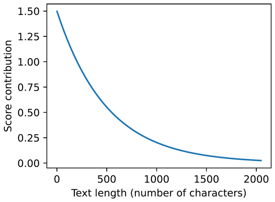 Figure 5.6 A simple rule-based length penalty used by our scorer. Longer explanations receive a smaller score contribution.
The score bonus approaches 1.5 for shorter answers, while answers longer than 1,000 characters receive a bonus of 0.2 or less.
For simplicity, the brevity bonus is computed using the number of characters rather than tokens, which avoids passing the tokenizer to the scoring function. Using token counts would also be reasonable (and may even be preferable).
We now apply the heuristic scorer to the first (longer) response from the previous section:
print(round(heuristic_score(response_1), 3))
The resulting score is 2.088. Next, let’s try the second (shorter) response:
print(round(heuristic_score(response_2), 3))
The computed score is 2.517, which means the second (shorter) response would be the preferred answer.
This section introduced the basic idea of scoring methods. Later in the chapter, we develop another scorer and return to the heuristic scorer when using it as part of the self-refinement method.
Sidebar: Exercise 5.1: Using the heuristic scorer as a tie-breaker in self-consistency
Extend the self-consistency implementation (
self_consistency_vote) in the previous chapter so that it can handle ties among the candidate answers. For instance, when two or more answers receive the same number of votes, apply the heuristic scorer (heuristic_score) from this section to the tied candidates and select the one with the highest score. Tip: You don’t need to modify theself_consistency_votefunction itself to apply the tie-breaking, but you can apply the tie-breaking to theself_consistency_votefunction’s returnedresultsdictionary.
Sidebar: Exercise 5.2: Using the heuristic scorer in a Best-of-N setup
Modify the self-consistency implementation so that the final answer is chosen using the heuristic scorer rather than majority voting. Generate N candidate answers for each problem (where N=2 or higher), score each candidate with the heuristic scorer, and select the one with the highest score as the final prediction. (If we use a scorer instead of majority vote, the method is called Best-of-N in the literature as opposed to self-consistency.)
Apply this method to a small subset of MATH-500 and compare the results to both plain Best-of-N and the self-consistency tie-breaker from the previous exercise.
Note that the scorer includes several parameters chosen by intuition, which is why we refer to it as a heuristic score. To optimize the extraction and brevity reward settings, we could plug this scorer into the self-consistency or Best-of-N methods from exercises 5.1 and 5.2 and evaluate which settings yield higher accuracy on a benchmark dataset such as MATH-500.
5.4 Understanding token probability scores
In this section, we take the first step toward building a scorer based on the model’s own confidence (step 5 in figure 5.7), where confidence means model-assigned probability. Specifically, in this section, we start by computing the token probability scores for a proposed answer and use them to estimate how likely the model considers that answer to be (step 3 in figure 5.7).
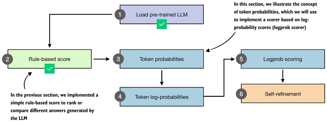 Figure 5.7 In this section, we move from a simple rule-based scorer to token-level probabilities. These probabilities form the basis for the logprob scoring method that we will use later in the self-refinement approach.
The token probability scores computed in this section are also known as next-token probabilities, per-token probabilities, sequence likelihoods, or loosely token-level likelihoods in the literature. They represent the probability the model assigns to each possible next token, expressed as a normalized (softmax) distribution over the vocabulary. Although this may sound complicated at first, it relies on the same mechanism used for text generation, which we covered in the previous chapter.
For instance, in the previous chapter, we saw that at each step the model assigns a so-called logit score to each token in the vocabulary and then selects the next token based on these scores. This process, which we discussed in section 4.4 of chapter 4, is illustrated again in figure 5.8 for reference.
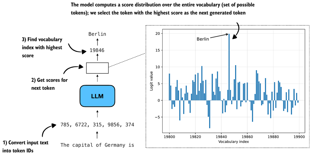 Figure 5.8 Illustration of how an LLM selects the next token. The model converts the input text into token IDs, computes a score for every vocabulary token, and chooses the token with the highest score. The plot on the right shows the logit values for a subset of the vocabulary, with the token for Berlin having the highest score.
In the previous chapter, we looked up the vocabulary entry corresponding to the highest score (vocabulary index 19846, corresponding to the token "Berlin" in figure 5.8), to get the next generated token.
Here, we revisit the logits with a different goal in mind. Instead of generating the next token as shown in figure 5.8, we want to use the scores to quantify the model’s confidence in a particular answer. In other words, we are not generating anything here based on the scores but are just inspecting the scores.
For example, consider two candidate answers we want to score:
"The capital of Germany is Berlin""The capital of Germany is Bridge"
The goal is to quantify how confident the model is in each answer.
In figure 5.8, the input text "The capital of Germany is" is fed to the model, and the next token with the highest score ("Berlin") is selected. Here, instead of selecting a token, we compare the scores assigned to two candidate next tokens, "Berlin" and "Bridge", as shown in figure 5.9. ("Bridge" is used as an alternative because it appears within the vocabulary range shown in figure 5.8.)
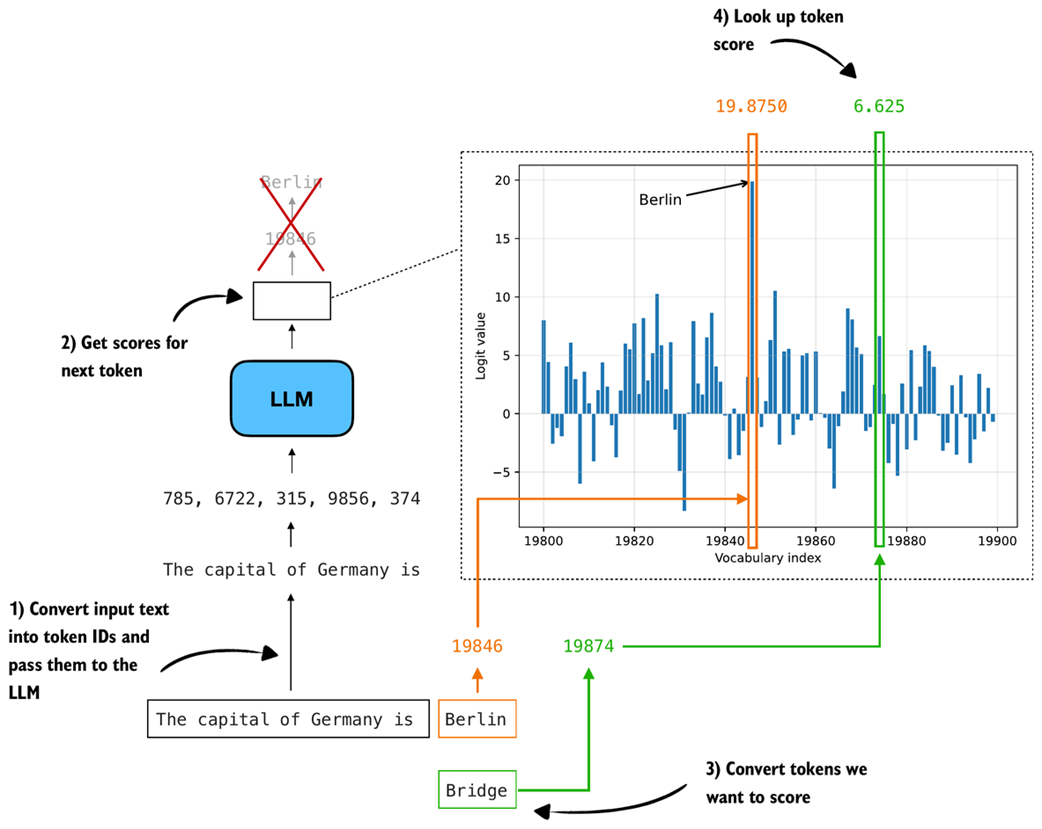 Figure 5.9 Illustration of how we look up the logit scores for specific tokens. After passing the input text through the model, we obtain a logit value for every vocabulary token. We then convert the candidate tokens we want to score into token IDs and read off their corresponding logit values from the distribution.
Rather than working with the raw logits shown in figure 5.9, we convert them to probabilities. Probabilities are easier to interpret, comparable across inputs, and form the basis for the logprob scoring method used later in the chapter.
As discussed in chapter 4, applying torch.softmax converts logits into probability values. Figure 5.10 shows the resulting probability distribution.
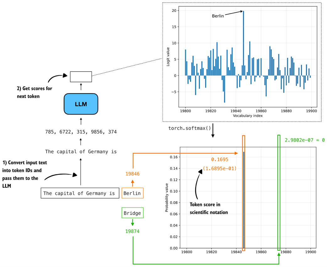 Figure 5.10 Illustration of next-token scoring. The input text is converted into token IDs and fed to the LLM, which outputs logits for the next token. After applying a softmax, these logits become probabilities, where tokens like “Berlin” receive high probability and unlikely alternatives such as “Bridge” receive values near zero.
The token probabilities shown in figure 5.10 are computed in the same way as in the previous chapter, using torch.softmax, as part of the multinomial sampling procedure described in section 4.4.3. The difference here is that we do not sample from the distribution. Instead, we simply look up the probability assigned to specific tokens.
In figure 5.10, only the bar for "Berlin" is visible, with a probability of 0.1695. The probabilities for other tokens in the plotted range are near zero. The bars shown do not sum to 1 because the full vocabulary contains 151,000 tokens, and the figure displays only a small slice of the distribution (token indices 19,800–19,900).
This indicates that the model assigns higher confidence to "Berlin" than to "Bridge" as the next token given the input text "The capital of Germany is".
In practice, however, we usually want to compare complete answers rather than individual tokens. This extension from single-token to sequence-level scoring is illustrated in figure 5.11.
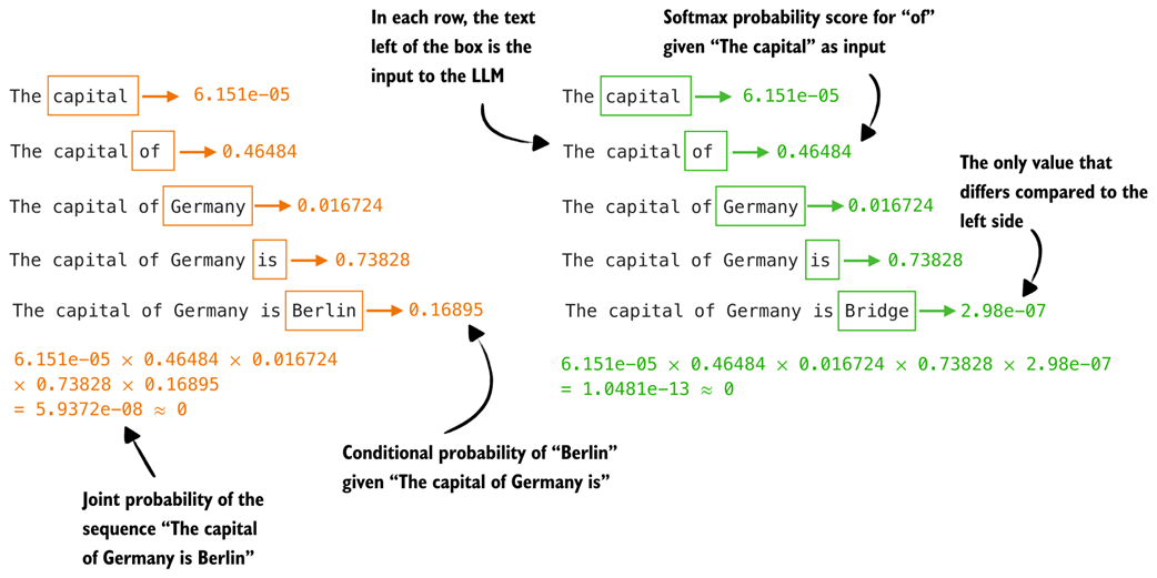 Figure 5.11 Illustration of how we compute token probability scores for a given sequence. For each position, we feed the preceding text into the model and read off the softmax probability of the next token. Multiplying these conditional probabilities yields the joint probability of the full sequence.
As shown in figure 5.11, we compute the probability of each token given its preceding tokens. This is the same procedure as in figure 5.10, except that we repeat it for every token in the sequence. Unlike text generation, we are not producing new tokens here. Instead, we retrospectively look up the probability assigned to each token in the already generated sequence.
We then multiply these probabilities to obtain the probability of the full sequence, also called the joint probability.
Sidebar: Joint probability of a token sequence
For those comfortable with mathematical notation, the joint probability of a token sequence can be written compactly as a product of conditional probabilities. For a sequence $x_1, x_2, …, x_T$ and model weights $W$, this is:
\[P(x_1, ..., x_T | W) = \prod_{t=1}^{T} P(x_t | x_{1:t-1}, W)\]Expanded, this becomes:
\[P(x_1, ..., x_T | W) = P(x_1 | W) \times P(x_2 | x_1, W) \times ... \times P(x_T | x_{1:T-1}, W)\]This matches exactly what we compute in figure 5.11. At each position we feed the context into the model, obtain the probability of the next token, and multiply these scores across the sequence.
Ideally, the probability assigned to the sequence "The capital of Germany is Berlin" should be much higher than that of the nonsensical answer "The capital of Germany is Bridge". However, because the joint probability is obtained by multiplying many small values, the resulting probabilities for both sequences in figure 5.11 are close to zero. We address this issue in the next section.
The two answers in figure 5.11 are nearly identical, differing only in the final token ("Berlin" versus "Bridge"), which we use here for simplicity and illustration. The same method can also be applied to sequences that differ more substantially, such as the answers generated earlier in this chapter for the MATH-500 prompt ("Half the value of $3x-9$ is $x+37$. What is the value of $x$?").
Sidebar: How this scoring differs from greedy and temperature plus top-p sampling
When we compute token probability scores, we are not generating text. The full sequence already exists, and we simply query the model for the probability of each next token given the fixed context as input. So, nothing about these probabilities influences later inputs. It is a retrospective scoring procedure, not a generation step.
Generation methods like the
generate_text_stream_cache(greedy sampling) andgenerate_text_top_p_stream_cachefunctions that we coded in chapter 4, behave very differently. Greedy sampling always selects the most likely next token, while temperature sampling and top-p sampling draw from a reshaped probability distribution. These procedures modify the distribution at each step and then commit to a single token, which becomes the input for the next position.An important consequence is that none of these sampling strategies, including greedy sampling, is guaranteed to produce the sequence with the highest overall probability under the model. A token that looks suboptimal at one step can lead to a future step where the following tokens are much more likely. On the other hand, a locally optimal choice may steer the model toward low-probability sequences later.
Temperature and top-p sampling add even more variability by flattening or truncating the distribution before drawing samples, which may further disconnect the generated text from the globally most likely sequence.
By scoring an existing answer, we avoid all these complications. We do not run a sampling algorithm and the model does not choose tokens. We only evaluate how probable the given sequence would have been if it had already been written.
After so much conceptual explanation, let’s now see the token probability calculation in action:
Listing 5.5 Calculating next token probabilities
@torch.inference_mode()
def calc_next_token_probas(model, tokenizer, prompt, device, show=True):

    token_ids = torch.tensor(tokenizer.encode(prompt), device=device)

    # Get logits and probabilities similar to text generation functions
    logits = model(token_ids.unsqueeze(0)).squeeze(0)
    all_probas = torch.softmax(logits, dim=-1)

    # Select positions we score (here: all)
    t_idx = torch.arange(0, token_ids.shape[0] - 1, device=device)

    # Since we have the text, we know the true next tokens
    next_ids = token_ids[1:]

    # Get probabilities for each next token
    next_token_probas = all_probas[t_idx, next_ids]

    prod_next_token_probas = torch.prod(next_token_probas)

    if show:
        print("Next-token probabilities:", next_token_probas)
        print("Joint probability:", prod_next_token_probas)

    else:
        return next_token_probas, prod_next_token_probas
As shown above, the calc_next_token_probas function, which computes the next-token probabilities as shown in figure 5.11, is relatively short and appears very simple at first glance. However, there’s a lot happening in this function to carry out the computation, as illustrated by a simpler input text example and a tiny five-word vocabulary in figure 5.12.
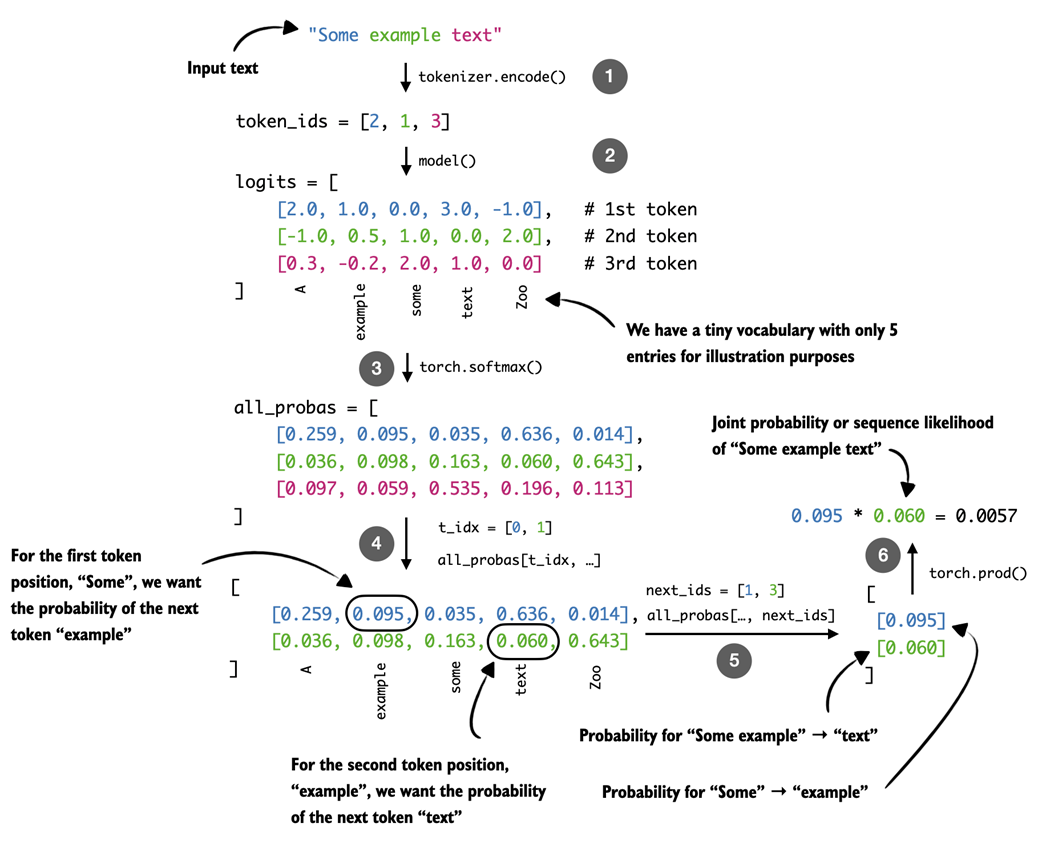 Figure 5.12 Illustration of how we extract next-token probabilities. After converting the input text into token IDs, the model computes logits that are transformed into probabilities with a softmax function. Using index tensors for positions and true next tokens, we then get the model’s computed probability for each next token.
The calc_next_token_probas function, illustrated with a simple example in figure 5.12, computes next-token probabilities in a few steps. First, it computes the logits in the same way as the text-generation functions introduced earlier (for example, the out = model(token_ids) line in generate_text_basic from chapter 2).
The resulting logits (step 2 in figure 5.12) have shape [sequence_length, vocab_size] and are then converted into normalized probability distributions using torch.softmax (step 3), so that the probabilities at each position sum to 1.
To extract the probability assigned to the actual next token at each position, we construct an index tensor t_idx for the positions we want to score and another tensor, next_ids, containing the corresponding target tokens. For example, if the input text is "The capital of Germany is Berlin", then t_idx refers to the positions corresponding to "The capital of Germany is", and next_ids contains the tokens shifted by one position: "capital of Germany is Berlin".
These target tokens are simply the input tokens shifted up by one position, since an LLM is trained to predict the next token in a sequence. For example, given the input "The capital of Germany is Berlin", the model is asked at position 2 (the token for "capital") to predict position 3 (the token for "of"). Using all_probas[t_idx, next_ids] (steps 4 and 5) retrieves exactly these probability values for each position in the sequence.
Finally, the function uses torch.prod to compute the sequence likelihood as the product of the per-token probabilities (step 6).
Let’s finally see this function in action:
torch.set_printoptions(precision=4)
calc_next_token_probas(
        model, tokenizer, device=device,
        prompt="The capital of Germany is Berlin"
    )
The resulting output is:
Next-token probabilities: tensor([6.1512e-05, 4.6484e-01,
1.6724e-02, 7.3828e-01, 1.6895e-01], dtype=torch.bfloat16)
Joint probability: tensor(5.9372e-08, dtype=torch.bfloat16)
Next, let’s try another text:
calc_next_token_probas(
        model, tokenizer, device=device,
        prompt="The capital of Germany is Bridge"
    )
This results in:
Next-token probabilities: tensor([6.1512e-05, 4.6484e-01, 1.6724e-02,
7.3828e-01, 2.9802e-07], dtype=torch.bfloat16)
Joint probability: tensor(1.0481e-13, dtype=torch.bfloat16)
Analyzing the results above, the first response (ending in "Berlin") gave us the joint probability (sequence likelihood) of 5.9372e-08, which is larger than the joint probability of the second response, 1.0481e-13. (In decimal form, 5.9372e-08 is 0.000000059372, and 1.0481e-13 is 0.00000000000010481.)
These results make sense since the "Berlin" answer receives a higher sequence likelihood than the "Bridge" answer, as expected. However, both values are extremely small because multiplying many small probabilities quickly produces numbers that approach zero. This makes raw likelihoods difficult to work with in practice, especially for longer sequences where underflow becomes a problem.
Note
These scores reflect the model’s internal likelihood, not a calibrated probability of correctness.
In the next section, we will introduce a modification to this calculation, log-probabilities, which avoid these numerical issues and give us a more stable way to score entire sequences.
Sidebar: Probabilities versus likelihoods
You may have noticed that this section used both terms, “probability” and “likelihood.” Is there a difference? In the field of statistics, probabilities describe how likely an event is before we observe any data and must sum to one across all possible outcomes. Likelihoods, in contrast, measure how well a specific model explains observed data and are viewed as a function of the model’s weights or parameters, not the data. In short, probabilities predict data given a model, while likelihoods evaluate models given data. (For a more detailed example, please see my article on probabilities versus likelihoods: https://sebastianraschka.com/faq/docs/probability-vs-likelihood.html)
In LLMs, the next-token probability is technically a probability, not a likelihood, because it comes from a normalized distribution over all possible next tokens that sums to one. In other words, the values in
next_token_probasare probabilities, not likelihoods. They come directly from the model’s softmax over the vocabulary for each position, which is a normalized probability distribution.The product, which is computed as the joint probability (
torch.prod(next_token_probas)), is the model’s probability assigned to the sequence. This quantity is often referred to as the sequence likelihood (especially when viewed as a function of the model parameters).
5.5 From token probability scores to log-probabilities
The token probabilities computed in the previous section can be used as a scoring function to rank different responses. However, as we saw, the probability scores can be very small, especially when multiplied to obtain the joint probability or sequence likelihood.
In this section, to avoid numerical stability issues that often arise when working with such small values, we apply a logarithmic scaling (also called log scaling) to these probabilities, as shown in the overview in figure 5.13.
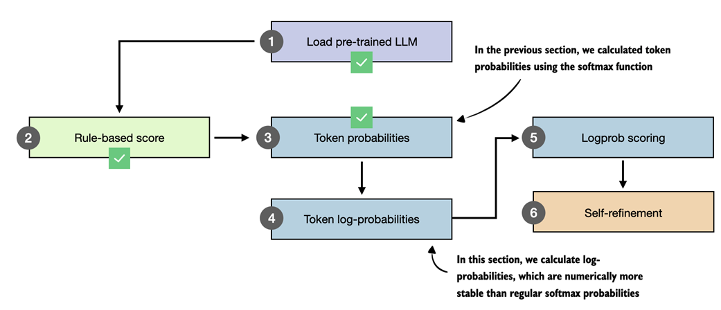 Figure 5.13 Overview of how we move from token probabilities to token log-probabilities, which provide a numerically more stable basis for log-probability scoring used later in self-refinement.
Note that this section is simply about applying a scaling transformation to the probabilities in the previous section, and the overall goal is still to compute the token probabilities, or, in this case, log-probabilities, as illustrated in figure 5.14.
For instance, consider this simple example computing the probabilities for a selection of logits values:
logits = torch.linspace(-2, 2, steps=7)
probas = torch.softmax(logits, dim=-1)
print(probas)
The probability values are:
tensor([0.0090, 0.0175, 0.0341, 0.0665, 0.1295, 0.2522, 0.4912])
We can turn them into log-probability scores via the torch.log function:
print(torch.log(probas))
The log-probability values are:
tensor([-4.7109, -4.0442, -3.3776, -2.7109, -2.0442, -1.3776, -0.7109])
Here, torch.log applies the mathematical, natural logarithm, where $\log(0.0090) = -4.7109$ and vice versa $e^{-4.7109} = 0.0090$.
Instead of chaining torch.log(torch.softmax(...)), PyTorch also has an optimized torch.log_softmax function that combines these two operations:
log_probas = torch.log_softmax(logits, dim=-1)
print(log_probas)
Similar to before, this returns:
tensor([-4.7109, -4.0442, -3.3776, -2.7109, -2.0442, -1.3776, -0.7109])
Note that the log-scaling only changes the magnitude of the values, not the ordering, so a sequence with a higher likelihood will always have a higher log-likelihood as well. To see this visually, let’s plot the logits, probabilities, and log-probabilities side by side:
Listing 5.6 Plotting logits, softmax probabilities, and log-softmax values
plt.figure(figsize=(9, 4))

# Plotting logits
plt.subplot(1, 3, 1)
plt.bar(range(len(logits)), logits, color="C0", alpha=0.7)
plt.title("Logits")
plt.xlabel("Token index")
plt.ylabel("Value")
plt.grid(alpha=0.3)

# Plotting softmax probabilities
plt.subplot(1, 3, 2)
plt.bar(range(len(probas)), probas, color="C1", alpha=0.7)
plt.title("torch.softmax(logits)")
plt.xlabel("Token index")
plt.ylabel("Probability")
plt.ylim(0, 1)
plt.grid(alpha=0.3)

# Plotting log-softmax values
plt.subplot(1, 3, 3)
plt.bar(range(len(log_probas)), log_probas, color="C2", alpha=0.7)
plt.title("torch.log_softmax(logits)")
plt.xlabel("Token index")
plt.ylabel("Log-probability")
plt.grid(alpha=0.3)

plt.tight_layout()
plt.savefig("logits_softmax_log_softmax.pdf")
plt.show()
The resulting plot is shown in figure 5.14.
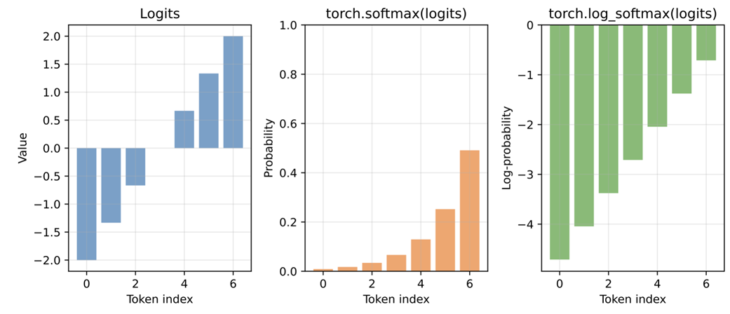 Figure 5.14 Comparison of logits, softmax probabilities, and log-probabilities for a simple example. The log-probabilities preserve the ordering of the probabilities.
As we can see in the resulting plot (figure 5.14), the log-probabilities have the same sorting order as the logits and probability values. A larger logit corresponds to a larger probability and a less negative log-probability. On the other hand, smaller logits produce smaller probabilities and more negative log-probabilities.
In practical terms, higher probabilities are better because they indicate the model assigns more confidence to a token. For log-probabilities, values closer to zero are better, since zero corresponds to a probability of one, while very negative values correspond to extremely small probabilities. This makes it easy to compare tokens: the least negative log-probability is the most likely one, and the most negative log-probability is the least likely.
While figure 5.14 illustrates the relationship between logits, probabilities, and log-probabilities for a simpler toy example, we can apply it to the probability values for the "The capital of Germany is" prompt example from earlier, as shown in figure 5.15.
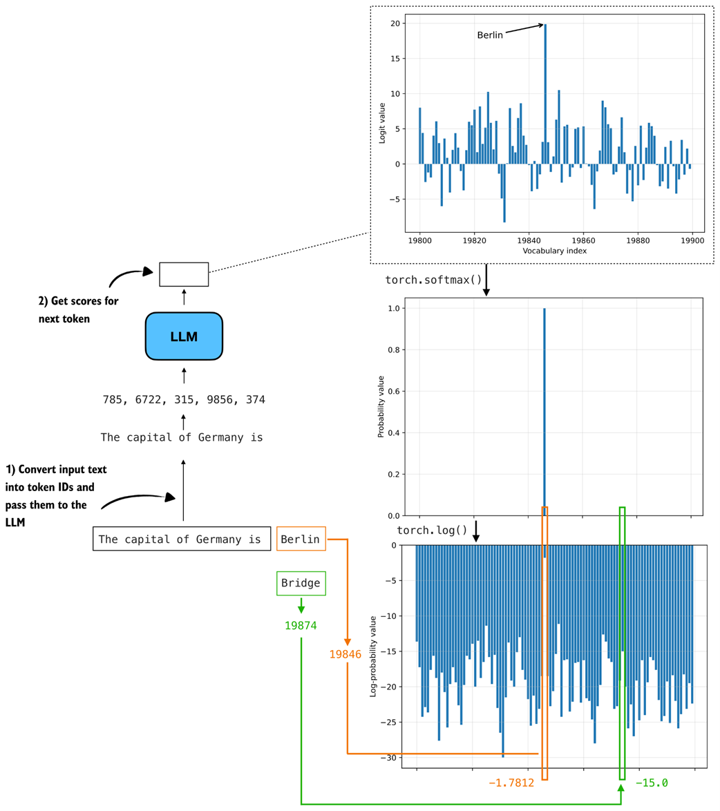 Figure 5.15 Illustration of how logits are converted to probabilities and log-probabilities for next-token scoring. The correct next token (“Berlin”) receives a high logit, which becomes a high probability and a less negative log-probability, while unlikely candidates like “Bridge” map to very small probabilities and large negative log-probabilities.
We use probabilities instead of logits because probabilities are normalized and easier to interpret as confidence values. Earlier we also noted that log-probabilities offer an additional benefit, since they allow for numerically more stable calculations than working with raw probabilities.
The numerical stability comes from the fact that even very small probability scores map to log-probabilities in a reasonable numeric range. The other reason is that multiplying many probabilities quickly drives the result toward zero, while taking the log turns this multiplication into addition, which avoids underflow and is much more stable for long sequences.
Figure 5.16 shows how the joint log-probability (or sequence log-likelihood) is computed for the two example texts we used earlier.
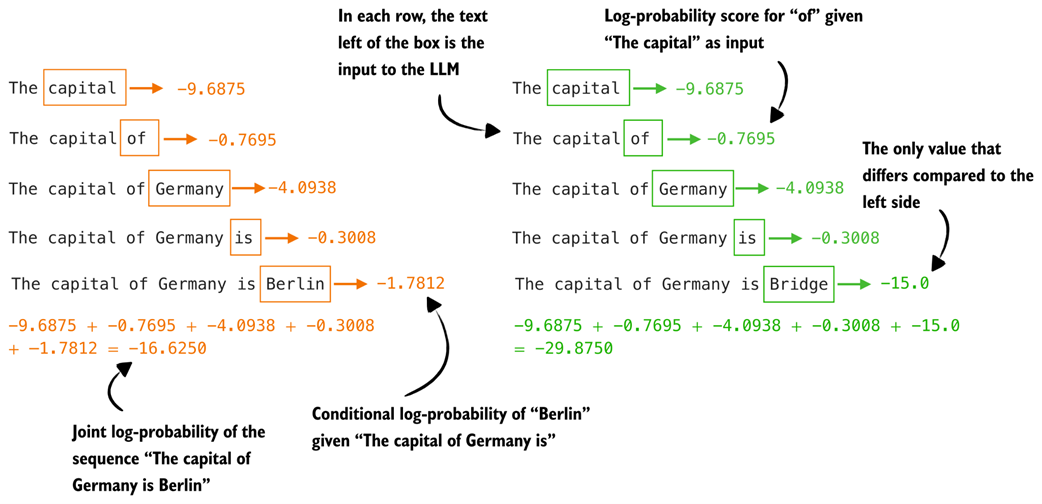 Figure 5.16 Illustration of how token-level log-probabilities accumulate to form sequence log-probabilities. Each row shows the log-probability of the next token given the preceding text. Summing these values results in the joint log-probability of the full sequence
Earlier, when we computed the regular joint probability score, we saw that both sequences had values close to zero. Now, with the joint log-probability, we can see in figure 5.16 that even changing just the final token (for example, "Berlin" versus "Bridge") results in a noticeably different total log-probability (-16.6250 versus -29.8750).
Sidebar: Working with log-probabilities
When we compute the joint probability of a sequence, we multiply many numbers between 0 and 1:
\[P(x_1, ..., x_T | W) = \prod_{t=1}^{T} P(x_t | x_{1:t-1}, W)\]In the expanded form, we can write it as:
\[P(x_1, ..., x_T | W) = P(x_1 | W) \times P(x_2 | x_1, W) \times ... \times P(x_T | x_{1:T-1}, W)\]These products quickly become extremely small, which is inconvenient and can cause numerical underflow. To avoid this, we often work in log space. Taking the logarithm of the joint probability gives:
\[\log P(x_1, ..., x_T | W) = \log \left( \prod_{t=1}^{T} P(x_t | x_{1:t-1}, W) \right)\]Using the fact that the logarithm of a product is the sum of the logarithms, this expands to:
\[\log P(x_1, ..., x_T | W) = \log P(x_1 | W) + \log P(x_2 | x_1, W) + ... + \log P(x_T | x_{1:T-1}, W)\]In other words, the log-probability of a sequence is just the sum of the log-probabilities of its individual tokens. This is both numerically more stable and easier to work with. It also matches the values returned by
torch.log_softmax, which provides the log-probabilities directly.Summing log-probabilities is therefore the standard approach in machine learning and AI.
Reusing the code from the previous section on calculating the token probabilities (listing 5.6), it is straightforward to implement the token log-probability function as it only requires two small changes: changing torch.softmax to torch.log_softmax and changing torch.prod to torch.sum.
Warning
Using mismatched combinations, such as
torch.softmaxwithtorch.sumortorch.log_softmaxwithtorch.prod, is technically possible but mathematically incorrect.
Listing 5.7 Calculating next token log-probabilities
@torch.inference_mode()
def calc_next_token_logprobas(model, tokenizer, prompt, device, show=True):

    token_ids = torch.tensor(tokenizer.encode(prompt), device=device)

    logits = model(token_ids.unsqueeze(0)).squeeze(0)

    # We now use log_softmax
    all_logprobas = torch.log_softmax(logits, dim=-1)

    t_idx = torch.arange(0, token_ids.shape[0] - 1, device=device)
    next_ids = token_ids[1:]
    next_token_logprobas = all_logprobas[t_idx, next_ids]

    # We replace the product with a sum
    sum_next_token_logprobas = torch.sum(next_token_logprobas)

    if show:
        print("Next-token log-probabilities:", next_token_logprobas)
        print("Joint log-probability:", sum_next_token_logprobas)
    else:
        return next_token_logprobas, sum_next_token_logprobas
Let’s now try the updated function on the example prompts from earlier:
calc_next_token_logprobas(
        model, tokenizer, device=device,
        prompt="The capital of Germany is Berlin"
    )
The result is:
Next-token log-probabilities: tensor([-9.6875, -0.7695, -4.0938,
-0.3008, -1.7812], dtype=torch.bfloat16)
Joint log-probability: tensor(-16.6250, dtype=torch.bfloat16)
And now the second sequence:
calc_next_token_logprobas(
        model, tokenizer, device=device,
        prompt="The capital of Germany is Bridge"
    )
This returns:
Next-token log-probabilities: tensor([ -9.6875,  -0.7695,  -4.0938,
-0.3008, -15.0000], dtype=torch.bfloat16)
Joint log-probability: tensor(-29.8750, dtype=torch.bfloat16)
As we can see, the difference between the "Berlin" and the "Bridge" sequence is now much more pronounced (-16.6250 and -29.8750), with the former scoring much higher (better).
5.6 Scoring model confidence with log-probabilities
The previous two sections explained the concepts of token probabilities and log-probabilities in great detail. In this section, we add some slight modifications to the log-probability computation to develop a log-probability-based scorer function analogous to the heuristic scorer we developed at the beginning of this chapter, as illustrated in figure 5.17.
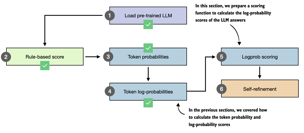 Figure 5.17 This section implements a logprob scorer, based on token log-probabilities, which we will use in the self-refinement method later in this chapter.
The logprob scoring method (logprob is a common term in the AI literature that is short for log-probability) we develop is very similar to the procedure we covered in the previous section. However, we make two main modifications.
First, we exclude the prompt from the score calculation and only calculate the score for the answer tokens. Second, we average (instead of summing) over the token log-probabilities so that it is fairer to compare two different sequences of different lengths. The updated calculation with these two modifications is shown in figure 5.18.
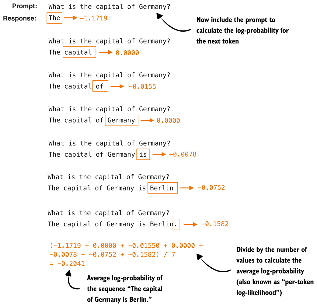 Figure 5.18 Illustration of the modified logprob scoring procedure. The prompt tokens are excluded from the calculation, and only the log-probabilities of the answer tokens are collected. These values are then averaged to obtain a length-normalized score, which allows us to compare answers of different lengths fairly.
For illustration purposes, we can implement the two modifications shown in figure 5.18 using the calc_next_token_logprobas function from the previous section. For example, suppose we have the following example prompt and answer:
example_prompt = "What is the capital of Germany?"
example_answer = " The capital of Germany is Berlin."

next_token_logprobas, sum_next_token_logprobas = calc_next_token_logprobas(
        model, tokenizer, device=device,
        prompt=example_prompt+example_answer,
        show=False
    )

print("Next-token logprobas:", next_token_logprobas)
print("Joint log-probability:", sum_next_token_logprobas)
This prints the following output:
Next-token logprobas: tensor([-0.4512, -0.3418, -8.3125, -0.3906,
-3.8125, -3.0469, -1.1719,  0.0000, -0.0155,  0.0000,
-0.0078, -0.0752, -0.1582], dtype=torch.bfloat16)
Joint log-probability: tensor(-17.7500, dtype=torch.bfloat16)
(Note that the tensor contains scores for the prompt token as well, which is why the numbers appear different from figure 5.18, but this will become more clear when you read on.)
We can then calculate the number of answer tokens via the following code, which yields 7:
print(len(tokenizer.encode(example_answer)))
Then, to calculate the average log-probability over the answer tokens, as shown in figure 5.18, we need to average over those 7 answer tokens:
last_7 = next_token_logprobas[-7:]
print(last_7)
print(torch.mean(last_7))

# This prints:
# tensor([-1.1719,  0.0000, -0.0155,  0.0000, -0.0078, -0.0752, -0.1582],
#        dtype=torch.bfloat16)
# tensor(-0.2041, dtype=torch.bfloat16)
We can see that the resulting average -0.2041 is similar to what’s shown in figure 5.18.
We can combine the calc_next_token_logprobas code with this calculation more conveniently into a new function, avg_logprob_answer, which is shown below:
Listing 5.8 Average log-probability scoring for answer tokens
@torch.inference_mode()
def avg_logprob_answer(model, tokenizer, prompt, answer, device="cpu"):

    # Encode prompt and answer tokens separately to get the prompt length later
    prompt_ids = tokenizer.encode(prompt)
    answer_ids = tokenizer.encode(answer)
    full_ids = torch.tensor(prompt_ids + answer_ids, device=device)

    # Same as in calc_next_token_logprobas before
    logits = model(full_ids.unsqueeze(0)).squeeze(0)
    logprobs = torch.log_softmax(logits, dim=-1)

    # Index range for positions corresponding to answer tokens
    start = len(prompt_ids) - 1
    end = full_ids.shape[0] - 1

    # Same as before, except for using start and end
    t_idx = torch.arange(start, end, device=device)
    next_tokens = full_ids[start + 1 : end + 1]
    next_token_logps = logprobs[t_idx, next_tokens]

    # Average over the answer token scores
    return torch.mean(next_token_logps)
The avg_logprob_answer function is overall similar to the calc_next_token_logprobas function from the previous section, except that we only calculate the logprob for the answer tokens, instead of the whole sequence including the prompt, and average over the calculated logprob values instead of summing them.
Let’s apply this new function to the prompt and answer from earlier in this section:
score_1 = avg_logprob_answer(
    model, tokenizer,
    prompt="What is the capital of Germany?",
    answer=" The capital of Germany is Berlin.",
    device=device
)
print(score_1)
This returns -0.2041 similar to before, which indicates that we implemented the function correctly. We can now also apply this function to the nonsensical "Bridge" answer:
score_2 = avg_logprob_answer(
    model, tokenizer,
    prompt="What is the capital of Germany?",
    answer=" The capital of Germany is Bridge.",
    device=device
)
print(score_2)
The resulting score here is -3.8906, much lower than the "Berlin" score, as expected.
With the average logprob scoring function in place, we could now also calculate the scores for the MATH-500 prompt (prompt_cot) we defined at the beginning of this chapter and the respective responses we stored as response_1 and response_2, which is left as an exercise for the reader.
We spend a lot of time in this chapter to go through the concepts of next-token probability and log-probability scoring. One reason for this is that we can use it as a scorer in the upcoming section on self-refinement. A second reason is that the concept of log-probabilities will also be relevant when we implement the reinforcement learning with verifiable rewards training in the upcoming chapter.
Sidebar: Exercise 5.3: Using the logprob scorer as a tie-breaker in self-consistency
Using the logprob scorer instead of the heuristic scorer in exercise 5.1, extend the self-consistency implementation (
self_consistency_vote) in the previous chapter so that it can handle ties among the candidate answers. Then run the two implementations on (a subset of) the MATH-500 dataset to see which tie-breaking method performs better.
Sidebar: Exercise 5.4: Using the logprob scorer in a Best-of-N setup
Extend the self-consistency implementation so that the final answer is chosen using the logprob scorer (
avg_logprob_answer) rather than the heuristic scorer or majority voting (similar to exercise 5.2). Then run the different implementations on (a subset of) the MATH-500 dataset to see which tie-breaking method performs better.Tip: You don’t need to modify the
self_consistency_votefunction itself to apply the tie-breaking, but you can apply the tie-breaking to theself_consistency_votefunction’s returnedresultsdictionary, which is used inside theevaluate_math500_streamfunction from chapter 3.
5.7 Self-refinement through iterative feedback
Having introduced several methods for scoring LLM answers, we now get to the core inference-scaling technique of this chapter, self-refinement (figure 5.19).
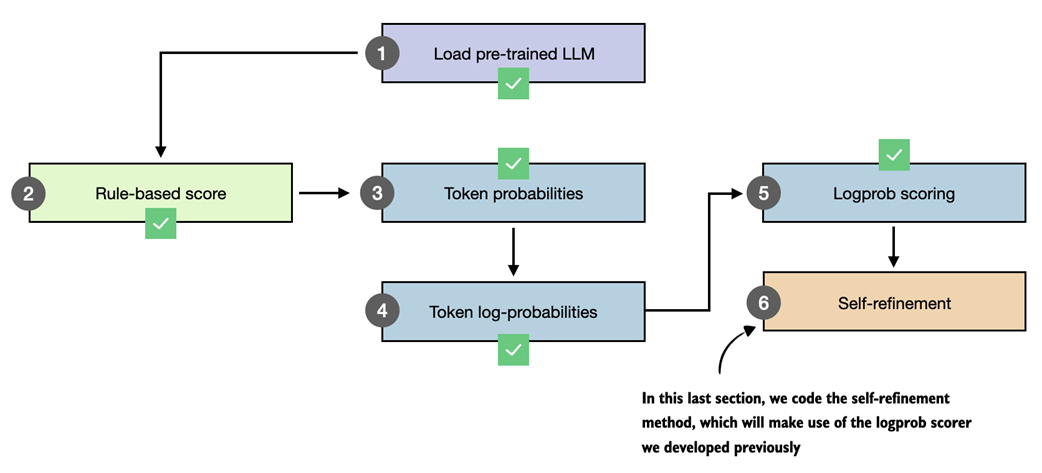 Figure 5.19 Overview of the final step in our workflow, where the logprob scorer developed earlier is used inside the self-refinement method.
This section introduces self-refinement and walks through the process manually for illustration. The next section, as shown in figure 5.19, then automates the self-refinement loop and adds support for the scoring methods developed earlier in the chapter (the heuristic scorer and the average logprob scorer).
Self-refinement is a technique in which the LLM analyzes and refines its own answers. As shown in figure 5.20, the LLM starts with an initial answer to the prompt as in regular LLM usage. Then, it critiques the answer and refines it.
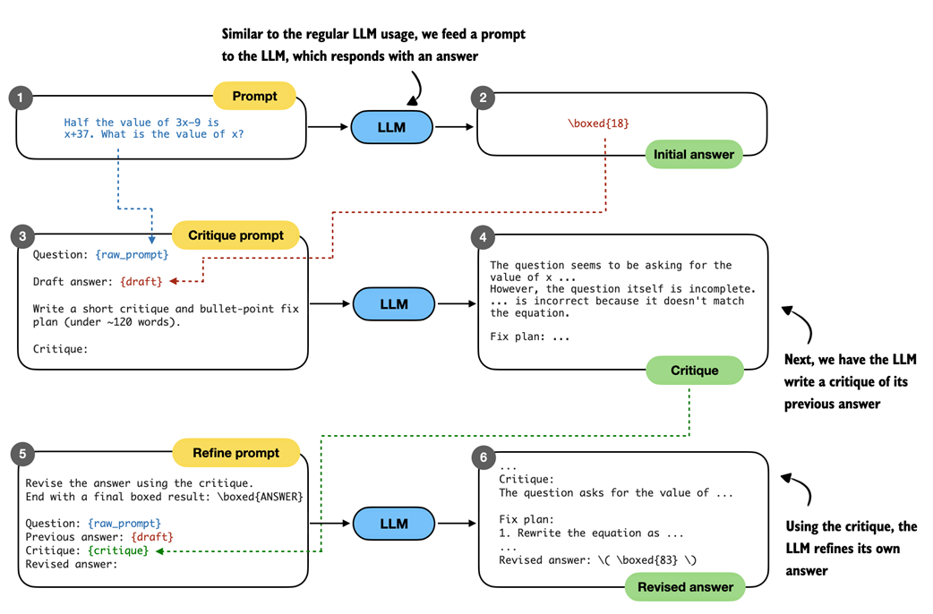 Figure 5.20 Illustration of the self-refinement process. The LLM first produces an initial answer to the prompt, then receives a critique prompt that asks it to analyze its own response and produce a short critique with a plan to refine the answer. In the final step, the model is given a refine prompt that contains the original question, its draft answer, and the critique, and it generates a revised answer that incorporates the suggested improvements.
The self-refinement procedure in figure 5.20 may look complicated at first, but it’s essentially just a sequential application of the error generation function on different prompts and inputs. To make it more clear, let’s walk through it step by step with a concrete code example.
Note
For this code example, we don’t use chain-of-thought prompting for illustration purposes. However, in practice, we can combine self-refinement with chain-of-thought prompting if we work with a base model.
We start with the base prompt and answer (steps 1 and 2 in figure 5.20), which is based on the code from section 5.2 at the beginning of this chapter, Loading a pre-trained model:
Listing 5.9 Base prompt and answer
raw_prompt = (
    "Half the value of $3x-9$ is $x+37$. "
    "What is the value of $x$?"
)
prompt = render_prompt(raw_prompt)

torch.manual_seed(123)
initial_response = generate_text_stream_concat_flex(
    model, tokenizer, prompt, device,
    max_new_tokens=2048, verbose=True,
    generate_func=generate_text_top_p_stream_cache,
    temperature=0.7,
    top_p=0.9,
)
The LLM responds with " \boxed{18}", which is an incorrect answer (the correct answer is 83).
Next, we have the LLM critique the answer. To do this we write a critique prompt, which includes the original question (raw_prompt) and answer (draft), as shown in steps 3 and 4 in figure 5.20. In code, this looks like as follows:
Listing 5.10 Critique prompt and refinement plan
def make_critique_prompt(raw_prompt, draft):
    return (
        "You are a meticulous reviewer. Identify logical errors, missing "
        "steps, or arithmetic mistakes. If the answer seems correct, "
        "say so briefly. Then propose a concise plan to fix issues.\n\n"
        f"Question:\n{raw_prompt}\n\n"
        f"Draft answer:\n{draft}\n\n"
        "Write a short critique and bullet-point fix plan "
        "(under ~120 words).\n"
        "Critique:"
    )


critique_prompt = make_critique_prompt(raw_prompt, initial_response)
torch.manual_seed(123)
critique = generate_text_stream_concat_flex(
    model, tokenizer, critique_prompt, device,
    max_new_tokens=2048, verbose=True,
    generate_func=generate_text_top_p_stream_cache,
    temperature=0.7,
    top_p=0.9,
)
The critique prompt above lets the LLM write an elaborate critique, which even contains the correct answer itself:
The question seems to have a logical error in its setup. The statement "Half the value of $3x-9$ is $x+37$" is incorrect because half of $3x-9$ should be $(3x-9)/2$, not $3x-9$. The equation should be $\frac{1}{2}(3x-9) = x + 37$.

Fix Plan:
1. Correct the equation to $\frac{1}{2}(3x-9) = x + 37$.
2. Multiply both sides by 2 to eliminate the fraction: $3x - 9 = 2(x + 37)$.
3. Distribute the 2 on the right side: $3x - 9 = 2x + 74$.
4. Subtract $2x$ from both sides: $x - 9 = 74$.
5. Add 9 to both sides: $x = 83$.
Note that the critique itself can contain factual errors, too, though. For instance, it says "The question itself is incomplete", which is not true, as it then proceeds with a correct fix plan. However, ultimately what matters is that the fix plan is correct.
Finally, we use this refinement prompt to revise the original answer (steps 5 and 6 in figure 5.20):
Listing 5.11 Answer refinement
def make_refine_prompt(raw_prompt, draft, critique):
    return (
        "Revise the answer using the critique. Keep it concise and "
        "end with a final boxed result: \\boxed{ANSWER}\n\n"
        f"Question:\n{raw_prompt}\n\n"
        f"Previous answer:\n{draft}\n\n"
        f"Critique:\n{critique}\n\n"
        "Revised answer:"
    )

refine_prompt = make_refine_prompt(raw_prompt, initial_response, critique)
torch.manual_seed(123)
revised_answer = generate_text_stream_concat_flex(
    model, tokenizer, refine_prompt, device,
    max_new_tokens=2048, verbose=True,
    generate_func=generate_text_top_p_stream_cache,
    temperature=0.7,
    top_p=0.9,
)
While the base model is not the best instruction-follower, the refinement prompt has the LLM generate the correct answer:
...
 \boxed{83}
Final result: The value of $x$ is \boxed{83}.
The procedure in this section illustrates a single refinement loop. In practice, it is not uncommon to repeat this loop for multiple iterations. In the next section, we will code a function to automate this process.
5.8 Coding the self-refinement loop
This final section packages the manual self-refinement steps from the previous section into a convenient function that simplifies using self-refinement and allows the process to be repeated for a fixed number of iterations.
In addition, the function supports plugging in the scoring methods developed earlier in the chapter (heuristic scoring and logprob scoring) to compute a score for each answer (figure 5.21), which can be used to decide whether a refined answer should be accepted.
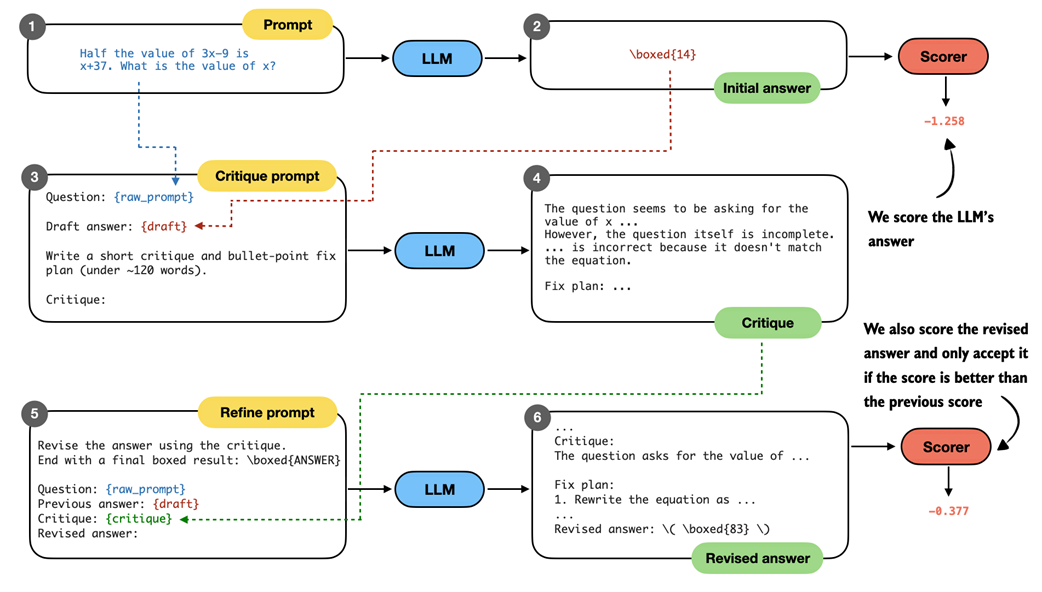 Figure 5.21 Overview of the self-refinement loop with optional scoring. The model first produces an initial answer, then critiques it, and generates a revised answer based on the critique. Both answers can be evaluated with the scoring functions from this chapter (for example, logprob scoring), and the revised answer is only accepted if its score improves on the previous one.
In figure 5.21, the revised answer receives a higher logprob score (-0.377) than the initial answer (-1.258), which makes it reasonable to accept the revision. In practice, however, self-refinement can also produce worse answers, especially when run for multiple iterations. The scorer therefore provides a way to decide whether a revised answer represents an improvement.
Note
Scoring does not always improve the results. Whether and which scorer to use in self-refinement depends on the LLM and needs to be figured out via experimentation on a benchmark dataset like MATH-500.
The complete code, which combines the steps from the previous section and adds an iterations parameter and a scoring function (score_fn) option, is shown in listing 5.12 below:
Listing 5.12 Self-refinement with multiple iterations and scoring support
def self_refinement_loop(
    model,
    tokenizer,
    raw_prompt,
    device,
    iterations=2,
    max_response_tokens=2048,
    max_critique_tokens=256,
    score_fn=None,
    prompt_renderer=render_prompt,
    prompt_suffix="",
    verbose=False,
    temperature=0.7,
    top_p=0.9,
):
    steps = []

    # Initial response (draft)
    prompt = prompt_renderer(raw_prompt) + prompt_suffix
    current_full = generate_text_stream_concat_flex(
        model=model,
        tokenizer=tokenizer,
        prompt=prompt,
        device=device,
        max_new_tokens=max_response_tokens,
        verbose=False,
        generate_func=generate_text_top_p_stream_cache,
        temperature=temperature,
        top_p=top_p,
    )

    current_extracted = extract_final_candidate(
        current_full, fallback="number_then_full"
    )
    if score_fn:
        current_score = score_fn(answer=current_full, prompt=prompt)
    else:
        current_score = 0.0

    # Run for one or more iterations
    for it in range(iterations):
        draft_before_full = current_full
        draft_before_extracted = current_extracted
        score_before = current_score

        # Critique the response
        critique_prompt = make_critique_prompt(
            raw_prompt, draft_before_full
        )
        critique_full = generate_text_stream_concat_flex(
            model=model,
            tokenizer=tokenizer,
            prompt=critique_prompt,
            device=device,
            max_new_tokens=max_critique_tokens,
            verbose=False,
            generate_func=generate_text_top_p_stream_cache,
            temperature=temperature,
            top_p=top_p,
        )

        # Refine the response
        refine_prompt = make_refine_prompt(
            raw_prompt, draft_before_full, critique_full
        )
        revised_full = generate_text_stream_concat_flex(
            model=model,
            tokenizer=tokenizer,
            prompt=refine_prompt,
            device=device,
            max_new_tokens=max_response_tokens,
            verbose=False,
            generate_func=generate_text_top_p_stream_cache,
            temperature=temperature,
            top_p=top_p,
        )

        revised_extracted = extract_final_candidate(
            revised_full, fallback="number_then_full"
        )
        if score_fn:
            revised_score = score_fn(
                answer=revised_full, prompt=prompt
            )
        else:
            revised_score = 0.0

        # Log the results
        step = {
            "iteration": it + 1,
            "draft_full": draft_before_full,
            "draft_extracted": draft_before_extracted,
            "critique": critique_full,
            "revised_full": revised_full,
            "revised_extracted": revised_extracted,
            "score_before": score_before,
            "score_after": revised_score,
        }
        steps.append(step)

        if verbose:
            print(
                f"[Refinement {it+1}/{iterations}]"
                f"\nCurrent: {draft_before_extracted}"
                f"\nRevised: {revised_extracted}"
                f"\nScore before: {score_before:.3f}"
                f"\nScore after: {revised_score:.3f}"
                f"\n{'=' * 25}\n"
            )

        # Accept revised response if it's not worse
        if revised_score >= current_score:
            current_full = revised_full
            current_extracted = revised_extracted
            current_score = revised_score

    return {
        "final_full": current_full,
        "final_extracted": current_extracted,
        "steps": steps,
    }
The self_refinement_loop function runs the self-refinement procedure from the previous section for one or more iterations (for it in range(iterations)). At the end of each iteration, it compares the revised score to the current score (revised_score >= current_score) and keeps the revised answer only if the score is equal or higher.
Using a scoring function is optional. When score_fn=None (the default), the score is always set to 0.0. Since 0.0 >= 0.0 evaluates to True, the most recent answer is always accepted when running multiple refinement iterations.
Next, we run the self-refinement loop using the average logprob scorer, avg_logprob_answer. The avg_logprob_answer function from listing 5.8 (section 5.6) takes several arguments (model, tokenizer, prompt, answer, and device). However, as shown in the previous listing, the scoring function is called with only two arguments:
# ...
        if score_fn:
            revised_score = score_fn(
                answer=revised_full, prompt=prompt
            )
# ...
To make avg_logprob_answer compatible with this score_fn call, we use the partial function from Python’s built-in functools module to pre-specify the remaining arguments:
Listing 5.13 Creating an average log-probability scorer
from functools import partial

avg_logprob_score = partial(
    avg_logprob_answer,
    model=model,
    tokenizer=tokenizer,
    device=device
)
Now, we can use the avg_logprob_score function in the self-refinement loop:
torch.manual_seed(1)

results_logprob = self_refinement_loop(
    model=model,
    tokenizer=tokenizer,
    raw_prompt=raw_prompt,
    device=device,
    iterations=2,
    max_response_tokens=2048,
    max_critique_tokens=256,
    score_fn=avg_logprob_score,
    verbose=True,
    temperature=0.7,
    top_p=0.9,
)
The output is shown below:
[Refinement 1/2]
Current: 10
Revised: 83
Score before: -0.855
Score after: -0.226
=========================
[Refinement 2/2]
Current: 83
Revised: 83
Score before: -0.226
Score after: -1.320
=========================
Looking at the results above, we see that the model corrected the initially incorrect answer (10 to 83) in the first iteration, and the score improved from -0.855 to -0.226. In the second iteration, the scores become worse, but that’s okay since we already have the correct answer.
We can also access the extracted number of the best-scoring answer via results_logprob["final_extracted"], which in this case returns 83. If you are interested in the full answer, use results_logprob["final_full"]. To read through the critiques and longer answers, you can print the results_logprob dictionary, which contains the detailed results for all iterations.
Sidebar: Exercise 5.5: Using the heuristic score for self-refinement
Run the
self_refinement_loopusing theheuristic_scorefunction, which we defined in section 5.3
The previous example showed that self-refinement can help the model with generating the correct answer. To get a better idea of how useful this self-refinement method really is, I ran this method on the MATH-500 from chapter 3 and summarized the results in table 5.1.
Table 5.1 MATH-500 task accuracy for different self-refinement methods
| Method | Scoring | Iterations | Model | Accuracy | Time | |
|---|---|---|---|---|---|---|
| 1 | Baseline (chapter 3) | - | - | Base | 15.2% | 10.1 min |
| 2 | Self-refinement | None | 1 | Base | 25.0% | 84.8 min |
| 3 | Self-refinement | None | 2 | Base | 22.0% | 165.4 min |
| 4 | Self-refinement | Heuristic | 1 | Base | 21.6% | 84.7 min |
| 5 | Self-refinement | Heuristic | 2 | Base | 20.8% | 151.4 min |
| 6 | Self-refinement | Avg. logprob | 1 | Base | 21.4% | 85.3 min |
| 7 | Self-refinement | Avg. logprob | 2 | Base | 22.0% | 165.3 min |
| 8 | Baseline (chapter 3) | - | - | Reasoning | 48.2% | 182.1 min |
| 9 | Self-refinement | None | 1 | Reasoning | 56.6% | 498.8 min |
| 10 | Self-refinement | Heuristic | 1 | Reasoning | 57.8% | 498.6 min |
| 11 | Self-refinement | Avg. logprob | 1 | Reasoning | 48.4% | 499.7 min |
The accuracy values shown in table 5.1 were computed on all 500 samples in the MATH-500 test set using a "cuda" GPU (A100 GPU).
As we can see in table 5.1, self-refinement improves the performance over the base model (rows 1-7). However, the improvement is only very moderate, with the best accuracy being achieved when no scoring is used in self-refinement. This means that both the heuristic score and average logprob score can sometimes lead to incorrect answers being accepted over the initial correct answer.
Note that when adding "Explain step by step." chain-of-thought for both the base model and the self-refinement, the model failed to improve over the base model (results not shown).
Looking at the reasoning model results (rows 8-11), we can see that the combination of self-refinement and heuristic scoring improved the answer accuracy by almost 10%. (As explained in chapter 3, the "reasoning" model can be used by changing which_model="base" to which_model="reasoning" in the load_model_and_tokenizer in section 5.2.)
In both cases, it seems that the average logprob scoring results in worse performance than no scorer or the heuristic scorer. This is likely because the logprob score favors answers that the model finds easy to produce rather than answers that are actually correct. Or, in other words, the logprob criterion can unintentionally select confident mistakes, whereas the heuristic score is more focused on the format and structure of the answer.
At this point, it seems we spent a lot of time discussing the average logprob scoring concept. However, logprob scoring is a fundamental concept when working with LLMs, and it will come handy in the upcoming chapters when we implement the reinforcement learning training procedure.
Comparing these results in table 5.1 with those from the previous chapter (table 4.1), we also observe that self-refinement is less effective than self-consistency for this model on this math task. Self-consistency remains widely used because it works well in practice, despite its simplicity.
Another method we have not explored in this chapter is self-refinement with an external model in an LLM-as-a-judge setup similar to what’s described in appendix B in section B.5. For instance, instead of using the heuristic score or average logprob, we use a second LLM to compute a score and to write the critique.
In November 2025, with DeepSeekMath-7B, the DeepSeek team demonstrated that self-refinement with a second LLM can be very successful, leading to gold-level performance in several math competitions. Specifically, the DeepSeek team proposed a new method in which they trained a second LLM to be a good critique model and further trained their base model to become a better math problem solver in the context of self-refinement (in contrast, in this chapter, we applied self-refinement without any additional training).
Speaking of inference and training, this chapter concludes the inference scaling without additional training (figure 5.22). In the next chapter, we begin covering training techniques that update the model weights to become better at reasoning tasks.
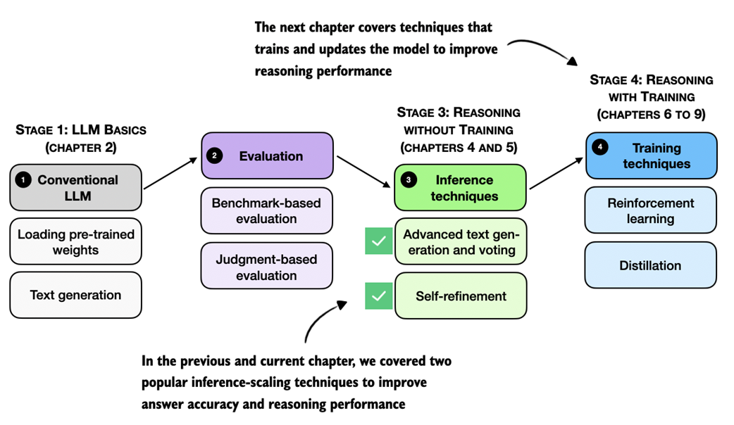 Figure 5.22 Overview of the book’s progression from basic LLM usage to inference-time reasoning methods and finally to training-based techniques. This chapter concludes the inference-scaling methods without additional training, and the next chapters introduce approaches that update model weights to further improve reasoning performance.
5.9 Summary
- Self-refinement extends the inference-time scaling ideas from the previous chapter by iteratively critiquing and improving a single answer instead of relying on multiple independent samples as in self-consistency.
- A simple rule-based scoring function ranks model outputs by rewarding extractable final answers and shorter, more economical completions.
- Next-token scoring quantifies model confidence by converting logits into normalized probabilities and combining these into a sequence-level likelihood.
- Log-probabilities replace raw probabilities to avoid numerical underflow and to turn products over many tokens into stable sums and averages.
- These scoring functions are more generally useful beyond self-refinement, for example, for breaking ties in self-consistency or implementing Best-of-N selection strategies.
- The self-refinement procedure consists of three stages: generating an initial draft, producing a short critique and fix plan, and generating a revised answer.
- A reusable refinement function automates the self-refinement workflow with multiple iterations (refinement rounds), and it can use a score-based acceptance to keep only revisions that do not degrade a computed answer score using one of the scoring functions we developed earlier.