Training reasoning models with reinforcement learning
Chapter 6: Training reasoning models with reinforcement learning
This chapter covers
- Training reasoning LLMs as a reinforcement learning problem with task-correctness rewards
- Sampling multiple responses per prompt to compute group-relative learning signals
- Updating the LLM weights using group-based policy optimization for improved reasoning
Reasoning performance and answer accuracy can be improved by both increasing the inference compute budget and by specific model training methods. This chapter, as shown in figure 6.1, focuses on reinforcement learning, which is the most commonly used training method for reasoning models.
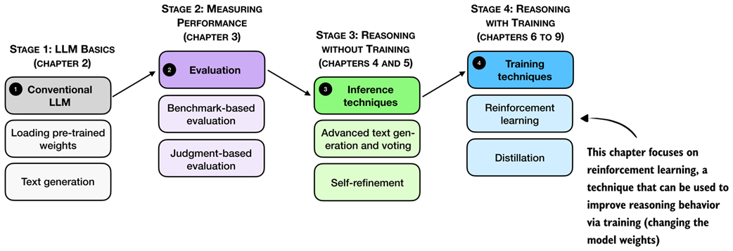 Figure 6.1 A mental model of the topics covered in this book. This chapter focuses on techniques that improve reasoning with additional training (stage 4). Specifically, this chapter covers reinforcement learning.
The next section provides a general introduction to reinforcement learning in the context of LLMs before discussing the two common reinforcement learning approaches used for LLMs.
6.1 Introduction to reinforcement learning for LLMs
Inference-time scaling and training-time scaling are two distinct approaches for improving the reasoning performance of large language models, as illustrated in figure 6.2. Inference-time scaling increases accuracy by spending more computation per generated answer, whereas training-time scaling improves accuracy by investing additional computation during training. This chapter focuses on training-time scaling.
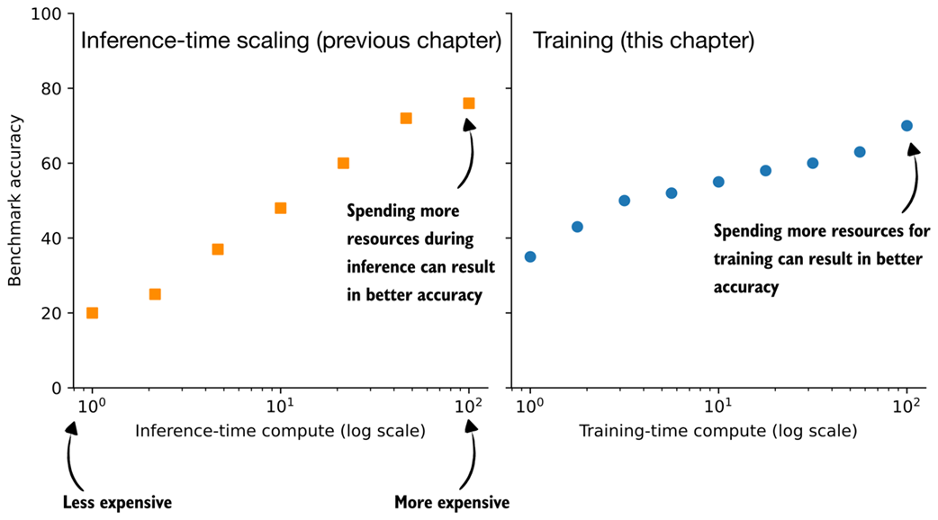 Figure 6.2 Conceptual comparison of inference-time scaling and training-time scaling. Increasing compute at inference improves accuracy by spending more resources per answer generation, while increasing compute during training improves accuracy by investing more resources upfront.
While figure 6.2 presents inference-time scaling and training-time scaling as separate concepts, in practice, both can be combined. For example, after improving a model’s reasoning capabilities through reinforcement learning (RL), which is the core focus of this chapter, inference-time scaling techniques such as those introduced in chapters 4 and 5 can be applied to further boost performance.
RL is focused on how models learn from sequences of actions and their outcomes, with classic examples such as agents trained to play Atari, Go, or video games.
While RL for LLMs builds on this literature, it differs in important ways and often resembles familiar LLM training techniques. Since this book focuses on language models, we do not cover RL in general but instead focus on how RL is applied in LLM training.
So what does RL mean in practice for LLMs? At a high level, RL is typically applied as a post-training stage on top of a pre-trained language model, sometimes after instruction fine-tuning. This setup is illustrated in figure 6.3.
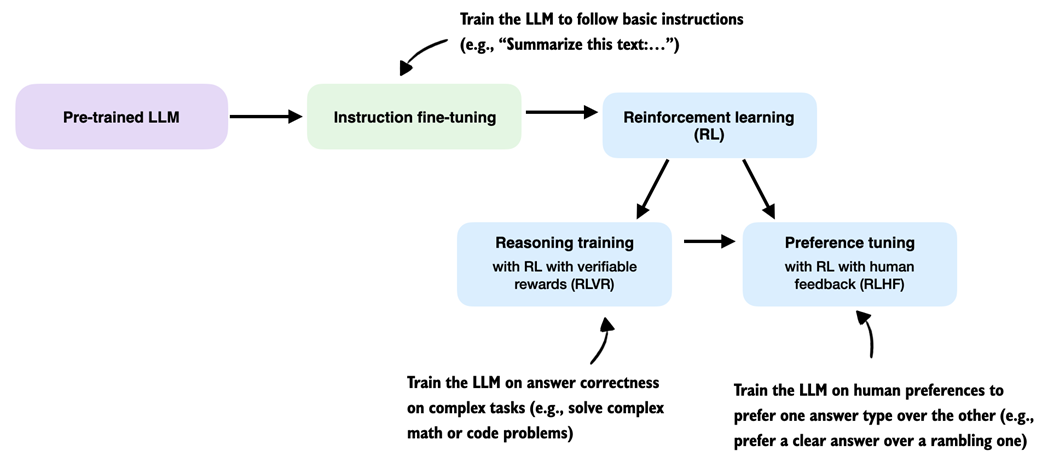 Figure 6.3 Common training stages for LLMs. The ordering of the reasoning training and preference tuning stages can vary, and some pipelines interleave reasoning and preference tuning rather than strictly sequencing them.
There are two common RL stages for LLMs: reasoning training and preference tuning. As shown in figure 6.3, RL is usually applied after instruction fine-tuning, and preference tuning often follows reasoning training. As demonstrated by the DeepSeek team in their DeepSeek-R1 work, though, reasoning-focused RL can also be applied directly to the pre-trained base model, skipping both instruction fine-tuning and preference tuning.
The resulting model is generally weaker in terms of reasoning accuracy than one that goes through the full training pipeline, but it still exhibits clear and robust reasoning behavior. More importantly, applying reasoning training directly to the base model avoids mixing the effects of multiple training stages, which makes it easier to attribute any observed improvements specifically to the reasoning training itself.
Before getting further into the details of how RL is implemented for LLMs, it is useful to briefly compare RL with pre-training at a conceptual level. During pre-training, an LLM is trained to predict the next token in large amounts of text, and many of the model’s core abilities and emergent behaviors (for example, answering knowledge-based questions and following simple instructions) already develop at this stage.
Note that pre-training is the main focus of my earlier book, Build a Large Language Model (From Scratch), but familiarity with that material is not required to follow this chapter or the rest of this book.
Applying RL on top of a pre-trained model is attractive because it lets us optimize whole outputs, such as answer correctness or preferences, rather than individual tokens and next-token prediction. In this sense, pre-training mainly builds knowledge, while RL shapes how the model uses that knowledge, including its reasoning behavior.
As shown in Figure 6.4, the next two subsections give a high-level overview of how RL is used in LLM training and set the context for the method used in this chapter.
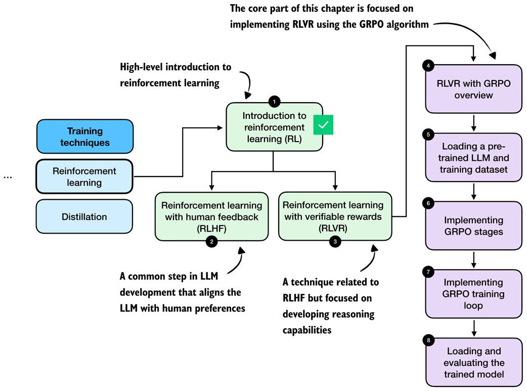 Figure 6.4 Roadmap of this chapter. After a brief introduction to reinforcement learning (RL) for LLMs in this section, we discuss the difference between two RL stages, RLHF and RLVR, in the next section. Then, we focus on implementing RLVR using the GRPO algorithm in the remainder of this chapter.
6.2 The original reinforcement learning pipeline with human feedback (RLHF)
In 2022, the InstructGPT paper (https://arxiv.org/abs/2203.02155) introduced reinforcement learning with human feedback (RLHF), a training approach that uses human preference labels to modify model behavior.
In fact, RLHF was a key ingredient in transforming GPT-3 into the original model used in ChatGPT, which was arguably what made LLMs broadly popular in 2022.
At a high level, RLHF is the most popular method to implement the preference tuning stage discussed in the previous section. Before RLHF, LLMs were primarily trained through pre-training and, in some cases, supervised fine-tuning, which are both based on next-token prediction objectives.
RLHF moved beyond this token-level optimization and optimizes models on the whole outputs (in this case, RLHF is optimizing for how humans rank and evaluate LLM outputs).
To make this more concrete, consider the following example. Suppose the prompt is: “I am looking to buy a laptop for programming and everyday use. What should I consider?”
The model might generate two candidate responses:
- Response A: “You should consider the CPU, RAM, storage, GPU, screen resolution, battery life, keyboard quality, port selection, thermal design, and price.”
- Response B: “For programming and everyday use, focus on a fast CPU, at least 16 GB of RAM, and an SSD with at least 256 GB storage. A comfortable keyboard and good battery life also matter. A GPU may only matter if you plan to train small LLMs locally.”
Both responses mention relevant points, but a human data annotator might prefer response B because it is more concrete and specific to the use case stated in the prompt.
In RLHF, such pairwise preferences are collected across many prompts and used to train the model to favor responses that humans consistently rank higher.
As shown in figure 6.5, RLHF has two main steps: (1) training a reward model (which is itself an LLM), and (2) using that reward model to score the target LLM outputs and fine-tune it.
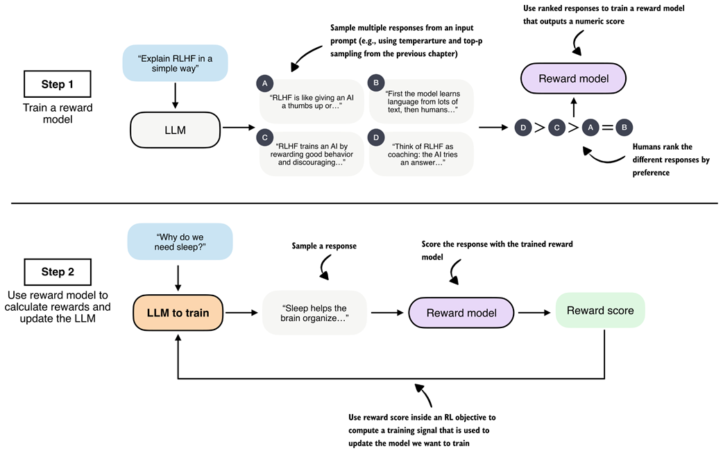 Figure 6.5 Two-stage overview of reinforcement learning with human feedback (RLHF). First, a reward model is trained on human-ranked responses to assign a preference score to each. Second, the LLM is updated using these reward scores within an RL objective to encourage preferred responses and discourage less desirable ones.
The first step in RLHF is training a reward model, as illustrated in the top subpanel of figure 6.5. Here, we have the LLM generate multiple responses per prompt (for example, using the temperature scaling and top-p filtering approach explained in chapter 4), and ask human annotators to rank the answers from best to worst based on their human preference.
These human preferences are converted into training targets for the reward model using a statistical preference model that maps pairwise comparisons into relative quality scores. The reward model, which is usually a separate model initialized from a pretrained LLM, is trained to output a single-number (scalar) reward score to each response that reflects its perceived quality.
The motivation is that the reward model can automatically score new model output, which eliminates the need for human annotation at every training step.
The second step in RLHF trains the LLM on the reward scores the reward model assigns to each of the LLM’s answers (for example, a bad answer may receive a -2, and a good answer may receive a +2).
We discuss RLHF here because it can be viewed as a precursor to reasoning-focused RL methods such as reinforcement learning with verifiable rewards (RLVR).
While the source of the training signal differs, human preferences versus automatically verifiable rewards, the underlying structure of the pipeline (generating responses, scoring them, and updating the model via RL) is closely related.
6.3 From human feedback to verifiable rewards (RLVR)
RLHF can be fairly involved because it requires training an additional reward model, which is often a large LLM that is (also) expensive to train.
Reinforcement Learning with Verifiable Rewards (RLVR) simplifies this setup by replacing the LLM reward model with verifiable rewards. Verifiable rewards are computed deterministically and without human annotation. For example, the math verifier introduced in chapter 3 is a verifiable reward generator for math problems.
For example, given a math problem (and a correct solution), a math verifier automatically checks whether a generated solution’s final answer matches the ground truth and assigns a corresponding reward (1 for correct, and 0 for incorrect responses).
As a result, the two-step RLHF pipeline collapses into a single training loop in RLVR, which resembles step 2 in RLHF: the model generates responses, the verifier assigns rewards, and these rewards are used directly to update the model.
This simplified RLVR training procedure is outlined in figure 6.6.
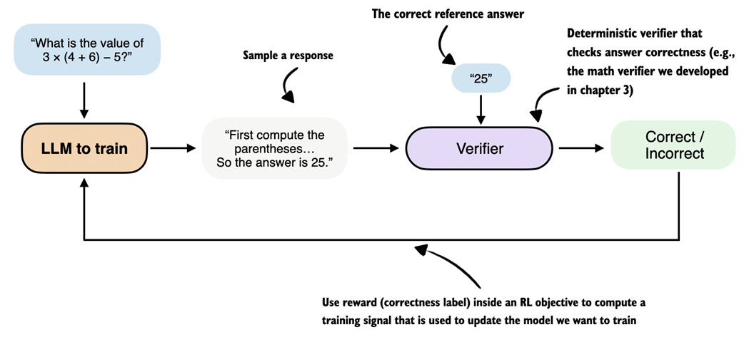 Figure 6.6 Overview of reinforcement learning with verifiable rewards (RLVR). The LLM generates a response that is evaluated by a deterministic verifier, for example the math verifier from chapter 3, which assigns a correctness label used as a reward signal within an RL objective to update the model.
The popularity of RLVR can largely be traced to the success of DeepSeek-R1 in 2025 (https://arxiv.org/abs/2501.12948), which demonstrated that strong reasoning performance can be achieved without relying on human preference data or a learned reward model.
DeepSeek-R1 trained reasoning behavior using automatically verifiable rewards, including correctness checks for math problems (similar to our verifier in chapter 3) and code compilation and execution for code-related tasks.
Code execution is outside the scope of this book, as this would require training the LLM in a secure environment, which further complicates things compared to solving math problems. The idea behind verifying math tasks (checking whether an answer is correct, as a binary label) and code compilation (checking whether code compiles, also as a binary label) is similar, and the RLVR training algorithm would be identical.
To summarize, RLVR offers several practical advantages over RLHF. It removes the need to train and maintain a separate reward model, which is often comparable in size and cost to the base LLM.
Verifiable rewards are also deterministic and reproducible, meaning they produce the same result every time for the same output, which avoids the noise and inconsistency that arise in human preference annotations.
Finally, RLVR scales naturally to large training sets, since, given a reference solution, rewards can be computed automatically for any number of model-generated answers without additional human labeling effort.
6.4 Reinforcement learning with verifiable rewards walkthrough using GRPO
Now that we have introduced the big picture and seen how RL fits within the overall development cycle of LLMs, we get to the concrete implementation. Specifically, we implement RLVR to train a reasoning model, as illustrated in the chapter roadmap in figure 6.7. This method is similar to DeepSeek-R1-Zero, but we apply it at a much smaller scale, on a smaller model with less data, since a comparable full training run would otherwise require several hundred thousand dollars in GPU compute.
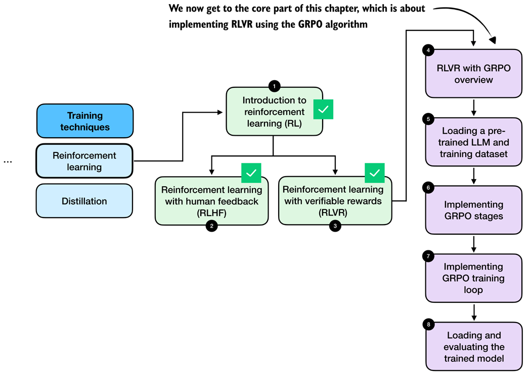 Figure 6.7 Chapter roadmap. After introducing the two main reinforcement learning approaches for LLMs, RLHF and RLVR, the remaining sections focus on implementing RLVR using the GRPO algorithm, from dataset loading to implementing the full training loop.
Note that RLVR defines the overall training setup, namely, using automatically verifiable rewards. In addition, we need a concrete policy optimization algorithm that can be used within this RLVR framework to update the model weights and train the model. The term “policy” is an RL-specific jargon and refers, in this specific context, to the LLM we want to train.
Specifically, we will use the group relative policy optimization (GRPO) algorithm for policy optimization.
In short, RLVR determines what learning signal is available, and GRPO determines how that signal is used to update the model weights.
Policy gradient algorithms
A widely used policy gradient algorithm for LLMs is proximal policy optimization (PPO), which was popularized in RLHF. In principle, the same algorithm could also be applied in an RLVR setting.
When training the DeepSeek-R1 reasoning models, the DeepSeek team opted for a simpler alternative, GRPO, which was originally introduced in their DeepSeekMath paper (https://arxiv.org/abs/2402.03300). GRPO is more resource-friendly than PPO because it does not require a separate value model to estimate a value function. Instead, GRPO derives its learning signal from relative comparisons within a group of sampled responses, which substantially reduces computational overhead.
Interested readers can find a more detailed side-by-side comparison of PPO and GRPO in my article The State of Reinforcement Learning for LLM Reasoning (https://magazine.sebastianraschka.com/p/the-state-of-llm-reasoning-model-training). In this chapter, we focus on implementing RLVR using GRPO, which is similar to what DeepSeek-R1 and other popular reasoning models use.
In the following chapter, we build on this foundation and introduce several practical extensions to GRPO that further improve training stability and the resulting reasoning performance.
6.5 High-level GRPO intuition via a chef analogy
The technical details of the GRPO algorithm for RLVR can be a bit overwhelming at first, since it has many moving parts and a lot of domain-specific RL terminology. So, before we start with a concrete technical overview and implementation, it may be beneficial to introduce the idea and mechanics behind GRPO with an example.
Figure 6.8 introduces the technical terms and approach of GRPO using a chef analogy preparing a meal.
 Figure 6.8 High-level overview of the GRPO algorithm for RLVR using a chef analogy. Multiple rollouts are generated and scored, relative advantages are computed, and a policy gradient objective with a KL-based regularization (loss) term is used to update the model parameters.
So, walking through the flowchart in figure 6.8, imagine we are a chef running a small food delivery service:
- Each day, we receive a single customer request (the prompt) asking us to prepare a certain dish (for example, lasagna).
- For that request, we cook our famous lasagna dish, but while doing so, we try out several different recipe variations (the rollouts).
- After preparing the recipes, we create multiple dishes (completions). Note in the LLM setting, a rollout refers to the entire generation process for a prompt, while the completion is the resulting output text. In practice, the two terms are often used interchangeably.
- Customers only give us feedback (the reward) after tasting the entire dish, not while it is being prepared. This means we judge the final result as a whole rather than individual cooking steps.
- We compare how the dishes performed relative to each other based on the customer feedback from stage 4. This helps us identify which recipe variations received higher rewards and which received lower rewards for this particular request.
- For each completed dish, we also keep track of how typical it was of our current cooking style, that is, how closely it followed our usual techniques and ingredient choices (logprobs).
- Using relative feedback from stage 5 and how characteristic each dish was of our current cooking style from stage 6, we determine how to tweak the cooking style (policy gradient loss). Here, we want to reinforce choices that led to better dishes and reduce those that led to worse ones.
- At the same time, we consult our original cookbook from the past.
- We then apply a style-preservation penalty that encourages trying new recipe variations, but prevents overly drastic changes to our cooking style that could scare away existing customers.
- The preference-based adjustment and the cooking style-preservation penalty are combined into a single overall measure or decision (the overall loss) about how the cooking style should change. The goal here is to balance customer satisfaction with consistency.
- Finally, we update the cooking style (gradient-based model weight update) so that future dishes are more likely to satisfy customer preferences while still remaining close to the original cookbook.
Even though this is a relatively intuitive analogy, we can see that there are lots of components and moving parts in GRPO.
6.6 The high-level GRPO procedure
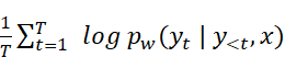
Following the food analogy from the previous section, the flowchart in figure 6.9 provides a technical overview of the GRPO algorithm for RLVR using concrete values and numbers that we will compute when implementing GRPO step by step.
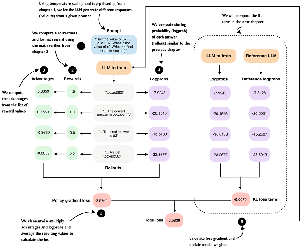 Figure 6.9 Step-by-step GRPO update for RLVR. (1) A prompt is sampled and multiple rollouts are generated. (2) Each rollout is scored using a verifiable reward. (3) Group-relative advantages are computed from these rewards. (4) The log-probability of each rollout under the current model is calculated. (5) Advantages and log-probabilities are combined to form the policy gradient loss. (6) A KL regularization term against a reference model is added, and the resulting total loss is used to update the model parameters.
The GRPO outline in figure 6.9 contains many technical components, and at first glance, it may look overwhelming. We will start by implementing a simplified version of GRPO that omits the KL loss term shown on the right side of the figure.
In chapter 7, we will add this missing KL loss term for completeness. While the KL loss is part of the original GRPO formulation, it is not strictly essential. In fact, many LLM developers omit it in practice, as doing so simplifies implementation and can sometimes improve modeling performance.
Note
Readers experienced with GRPO or other policy gradient methods may wonder about the use of clipped policy ratios; these are covered in the upcoming chapter.
If this overview, shown in figure 6.9, feels complicated on first reading, don’t worry. We will build up the algorithm step by step. For now, it is best to treat figure 6.9 as a high-level roadmap that helps orient ourselves as we work through the individual pieces.
6.7 Loading a pre-trained model
Similar to previous chapters, we begin by loading the pre-trained model (see stage 5 in figure 6.10), which we will then use to generate the rollouts (answers to a given prompt) we need for GRPO.
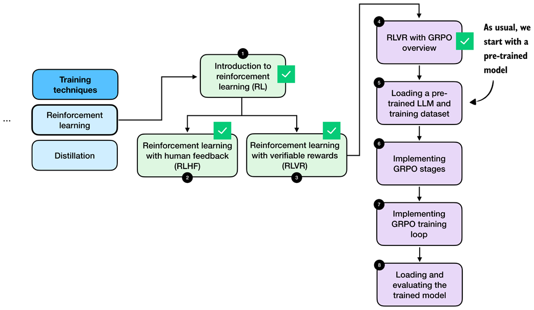 Figure 6.10 In stage 5, we load the pre-trained model (this section) and dataset (next section) that we will use for the model training.
Listing 6.1 is the same code we’ve used previously for loading the tokenizer and base model.
Listing 6.1 Loading tokenizer and base model
import torch
from reasoning_from_scratch.ch02 import get_device
from reasoning_from_scratch.ch03 import (
     load_model_and_tokenizer
)

device = get_device()
device = torch.device("cpu")

model, tokenizer = load_model_and_tokenizer(
    which_model="base",
    device=device,
    use_compile=False
)
Note: Delete the line device = torch.device("cpu") to run the code on a GPU (if supported by your machine).
Note that the code in listing 6.1 sets the CPU by default to ensure you get results that are more consistent with what’s shown in this chapter. Once you have done a full pass through this chapter, I recommend deleting the line device = torch.device("cpu") and running the chapter code on a GPU.
Next, to ensure that the model is loaded correctly, let’s use it together with the temperature and top-p sampler code from chapter 4 on a simple math prompt:
Listing 6.2 Generating text with temperature scaling and top-p sampling
from reasoning_from_scratch.ch03 import render_prompt
from reasoning_from_scratch.ch04 import (
    generate_text_stream_concat_flex,
    generate_text_top_p_stream_cache
)

raw_prompt = (
    "Half the value of $3x-9$ is $x+37$. "
    "What is the value of $x$?"
)
prompt = render_prompt(raw_prompt)

torch.manual_seed(0)
response = generate_text_stream_concat_flex(
    model, tokenizer, prompt, device,
    max_new_tokens=2048, verbose=True,
    generate_func=generate_text_top_p_stream_cache,
    temperature=0.9,
    top_p=0.9
)
print(response)
The model prints " \boxed{58}", which is an incorrect answer (83 is correct), but that’s okay since the goal here was merely to make sure that the code runs without issue.
6.8 Loading a MATH training subset
Next, we load the dataset that we will use when training the model with GRPO.
We use a non-overlapping training subset derived from the original MATH dataset, which means that all MATH-500 evaluation problems are explicitly excluded from the training data. This prevents data leakage and ensures a clean separation between training and evaluation, as illustrated in figure 6.11.
Note
For details on how this dataset was constructed, see https://github.com/rasbt/math_full_minus_math500.
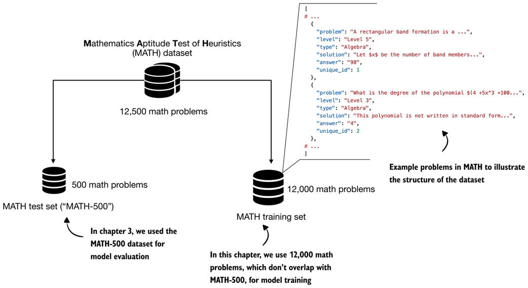 Figure 6.11 Structure and split of the MATH dataset. The full dataset contains about 12,500 problems that are divided into a 500-problem test set (MATH-500), which we used for model evaluation in chapter 3. A non-overlapping set of 12,000 problems is used for training in this chapter.
To load the 12,000 math problems from the MATH training set depicted in figure 6.11, we define the following load_math_train function in listing 6.3, which is similar to the load_math500_test function in chapter 3, except that we specify a different file path.
Listing 6.3 Loading the MATH training set
import json
from pathlib import Path
import requests

def load_math_train(local_path="math_train.json", save_copy=True):
    local_path = Path(local_path)
    url = (
        "https://raw.githubusercontent.com/rasbt/"
        "math_full_minus_math500/refs/heads/main/"
        "math_full_minus_math500.json"
    )

    if local_path.exists():
        with local_path.open("r", encoding="utf-8") as f:
            data = json.load(f)
    else:
        r = requests.get(url, timeout=30)
        r.raise_for_status()
        data = r.json()

        if save_copy:  # Saves a local copy
            with local_path.open("w", encoding="utf-8") as f:
                json.dump(data, f, indent=2)

    return data

math_train = load_math_train()
print("Dataset size:", len(math_train))
The above code should print "Dataset size: 12000" to indicate that the dataset was loaded correctly.
Next, we can also print one of the 12,000 entries to get an idea of the dataset structure. For this, we use the pprint function from the pprint standard library, as it provides nicer formatting for dictionary entries compared to the regular print function:
from pprint import pprint
pprint(math_train[4])
The resulting entry (index 4 corresponds to the fifth entry in the dataset) is shown below:
{
    "answer": "6",
    "level": "Level 3",
    "problem": (
        "Sam is hired for a 20-day period. On days that he "
        "works, he earns $\\$60. For each day that he does "
        "not work, $\\$30 is subtracted from his earnings. "
        "At the end of the 20-day period, he received "
        "$\\$660. How many days did he not work?"
    ),
    "solution": (
        "Call $x$ the number of days Sam works and $y$ the "
        "number of days he does not... Thus, Sam did not "
        "work for $\\boxed{6}$ days."
    ),
    "type": "Algebra",
    "unique_id": 4,
}
As we can see, each dataset example is stored as a dictionary with several fields. For training, the relevant fields are "problem", which serves as the prompt, and "answer", which is the target we verify the model’s output against using the math verifier.
The dataset also includes a full worked solution in the "solution" field. While such step-by-step solutions could in principle be used to evaluate intermediate reasoning steps, doing so would unnecessarily constrain the model and risk overfitting to a specific solution and style. Instead, we want to allow the model to explore the solution space more freely.
6.9 Sampling rollouts
After setting up the pre-trained base model and loading the dataset we are now ready to implement the GRPO stages, as illustrated in figure 6.12.
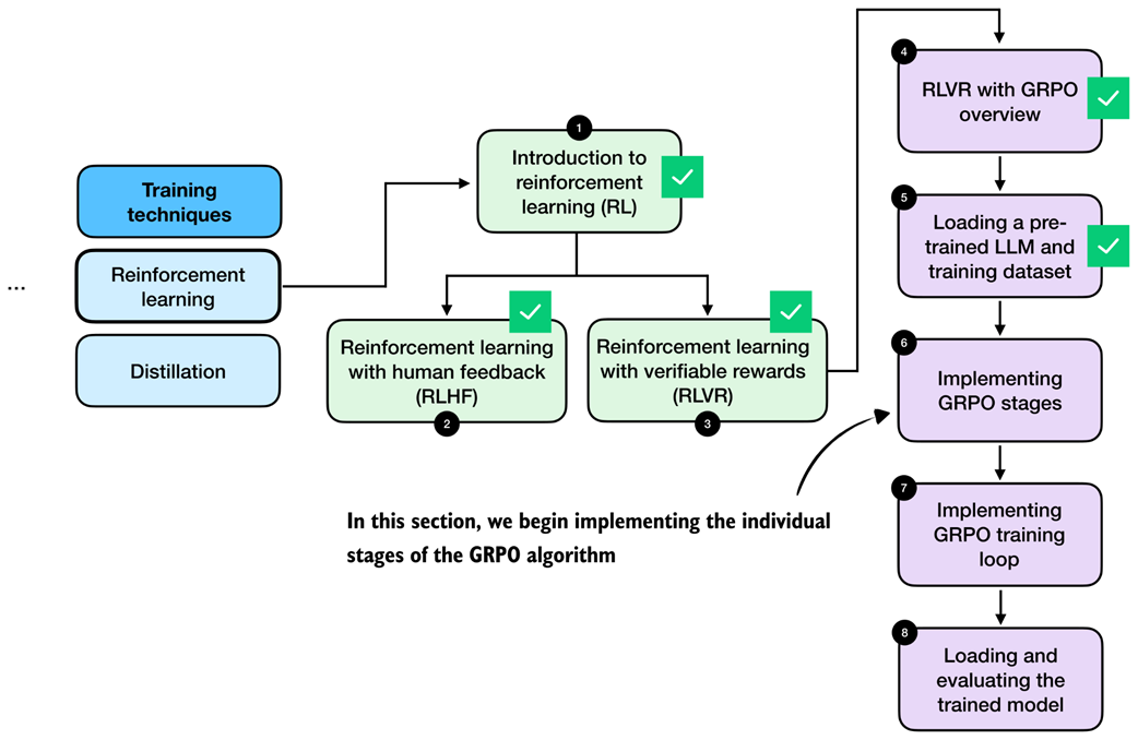 Figure 6.12 After outlining the RLVR method and GRPO algorithm, the following sections implement the individual GRPO stages that we need to train the LLM via verifiable rewards on the MATH dataset.
Before we begin, figure 6.13 revisits the GRPO overview introduced earlier, but in a simplified form that omits the KL loss term, which we will add in the next chapter. Referring back to this overview will help us orient ourselves as we work through the algorithm’s components.
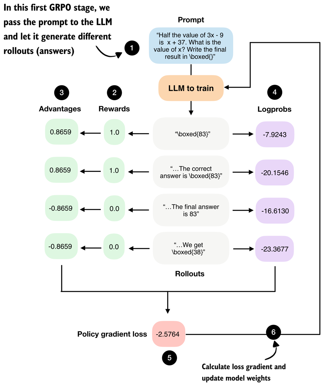 Figure 6.13 Step-by-step GRPO update for RLVR (without KL loss term). We begin by prompting the LLM to generate the different rollouts.
As shown in figure 6.13, we first use the LLM to generate multiple rollouts. Here, “rollout” is a reinforcement learning term that simply refers to a complete answer generated by the model for a given prompt.
We could reuse the generate_text_stream_concat_flex function from listing 6.2 to generate the rollouts. When we defined that function earlier, though, we decorated it with @inference_mode, which disables several PyTorch features for efficiency. Since we will later perform a backward pass, this makes the function incompatible with our training setup. Instead, we need to use the @torch.no_grad decorator, which disables gradient tracking for the forward pass without switching PyTorch into inference-only mode.
Let’s rewrite the function in a more compact form and call it sample_response. Importantly, this function generates text identical to generate_text_stream_concat_flex(..., generate_func=generate_text_top_p_stream_cache). We can verify this by observing that, with the same random_seed, temperature, and top_p settings, both functions produce identical generated responses.
Listing 6.4 Defining the rollout generation function
from reasoning_from_scratch.qwen3 import KVCache
from reasoning_from_scratch.ch04 import top_p_filter


@torch.no_grad()
def sample_response(
    model,
    tokenizer,
    prompt,
    device,
    max_new_tokens=512,
    temperature=0.8,
    top_p=0.9,
):
    input_ids = torch.tensor(
        tokenizer.encode(prompt),
        device=device
        )

    cache = KVCache(n_layers=model.cfg["n_layers"])
    model.reset_kv_cache()
    logits = model(input_ids.unsqueeze(0), cache=cache)[:, -1]

    generated = []
    for _ in range(max_new_tokens):
        if temperature and temperature != 1.0:
            logits = logits / temperature

        probas = torch.softmax(logits, dim=-1)
        probas = top_p_filter(probas, top_p)
        next_token = torch.multinomial(
            probas.cpu(), num_samples=1
        ).to(device)

        if (
            tokenizer.eos_token_id is not None
            and next_token.item() == tokenizer.eos_token_id
        ):
            break
        generated.append(next_token.item())
        logits = model(next_token, cache=cache)[:, -1]

    full_token_ids = torch.cat(
        [input_ids,
         torch.tensor(generated, device=device, dtype=input_ids.dtype),]
    )
    return full_token_ids, input_ids.numel(), tokenizer.decode(generated)
Note that the function now also returns the token IDs of the prompt plus answer tokens and the number of tokens (input_ids.numel()) next to the answer text (tokenizer.decode(generated)). Returning these allows us to simplify several downstream functions later on.
Otherwise, there is nothing new here. The code is simply a leaner version of what we’ve been developing previously; it combines the generate_text_basic_stream_cache function from chapter 2 with temperature and top-p sampling from chapter 4 directly.
Next, we call the function on an example prompt similar to listing 6.2.
Listing 6.5 Generating rollouts with temperature scaling and top-p sampling
torch.manual_seed(0)

raw_prompt = (
    "Half the value of $3x-9$ is $x+37$. "
    "What is the value of $x$?"
)
prompt = render_prompt(raw_prompt)

token_ids, prompt_len, answer_text = sample_response(
            model=model,
            tokenizer=tokenizer,
            prompt=prompt,
            device=device,
            max_new_tokens=512,
            temperature=0.9,
            top_p=0.9,
        )

print(answer_text)
Similar to before, the function returns " \boxed{58}".
Note, we could call sample_response multiple times to generate different rollouts, which we will indeed do later when implementing the full training loop. For now, to keep the GRPO walkthrough example simple and to make it easier to follow the step-by-step GRPO outline from figure 6.13, we instead assume that the model produced the following four short responses:
rollouts = [
    r"\boxed{83}",
    r"The correct answer is \boxed{83}",
    r"The final answer is 83",
    r"We get \boxed{38}",
]
6.10 Calculating rewards
The second stage of the GRPO procedure involves computing rewards for each rollout, as shown in figure 6.14.
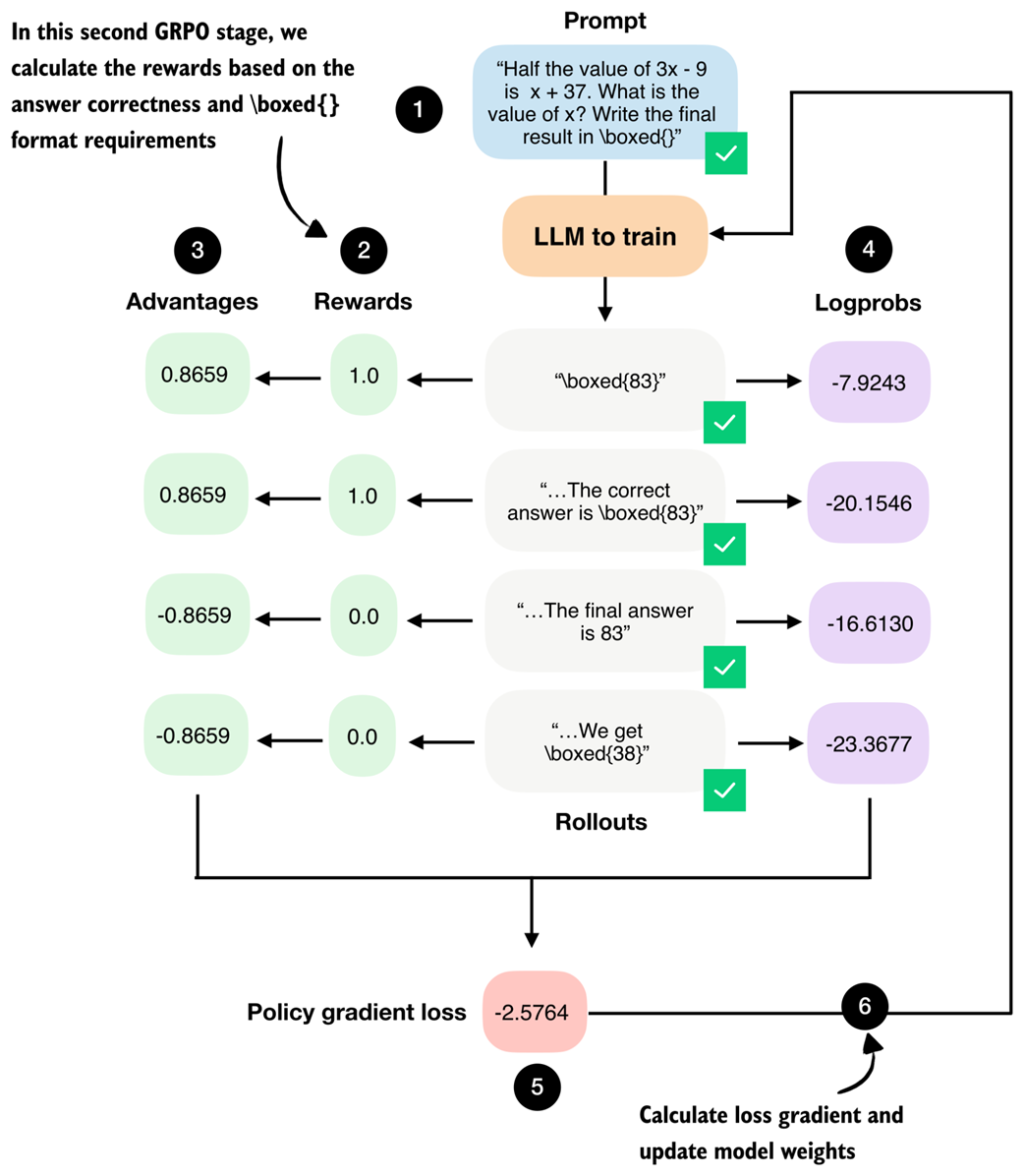 Figure 6.14 The second stage in the GRPO pipeline computes the rewards for each rollout the LLM generated in the previous section.
The rewards are computed using the math verifier from chapter 3 and are primarily based on answer correctness. By setting fallback=None in the reward_rlvr function in listing 6.6, we also include an implicit format constraint. For instance, an answer only receives a reward of 1.0 if it is both correct and expressed in the required \boxed{} format.
Listing 6.6 Implementing the reward function
from reasoning_from_scratch.ch03 import (
    extract_final_candidate, grade_answer
)

def reward_rlvr(answer_text, ground_truth):
    extracted = extract_final_candidate(
        answer_text, fallback=None
    )
    if not extracted:
        return 0.0
    correct = grade_answer(extracted, ground_truth)
    return float(correct)
Since the model receives a non-zero reward only if it answers correctly and writes the final answer in the \boxed{} format, we encourage it to learn to produce correct and properly formatted answers.
Let’s give the reward_rlvr function a try and apply it to the rollouts.
Listing 6.7 Applying the reward function to all rollouts
rollout_rewards = []

for answer in rollouts:
    reward = reward_rlvr(answer_text=answer, ground_truth="83")
    print(f"Answer: {answer!r}")
    print(f"Reward: {reward}\n")
    rollout_rewards.append(reward)
The resulting outputs are as follows:
Answer: '\\boxed{83}'
Reward: 1.0

Answer: 'The correct answer is \\boxed{83}'
Reward: 1.0

Answer: 'The final answer is 83'
Reward: 0.0

Answer: 'We get \\boxed{38}'
Reward: 0.0
As shown above, the reward function works as intended and only provides a reward of 1.0 if the answer contains the correct result (83) and uses the \boxed{} format.
Note that the DeepSeek-R1 team also tried to use process reward models to score intermediate solution steps during training. These attempts were unsuccessful, and the researchers concluded that it is better to train only on final-answer correctness rewards, without intermediate rewards.
Exercise 6.1: Adding format-aware reward shaping
Extend the
reward_rlvrfunction from this chapter so that it assigns partial credit based on output format. Specifically, modify the reward function so that it returns1.0if the model produces the correct answer in the required\boxed{}format,0.5if the answer is correct but not boxed, and0.0otherwise.
6.11 Preparing learning signals from rollouts via advantages
We now move on from rewards to the so-called advantages, as shown in figure 6.15. While rewards tell us how well each individual rollout performed, advantages capture how a rollout performed relative to other rollouts generated for the same prompt.
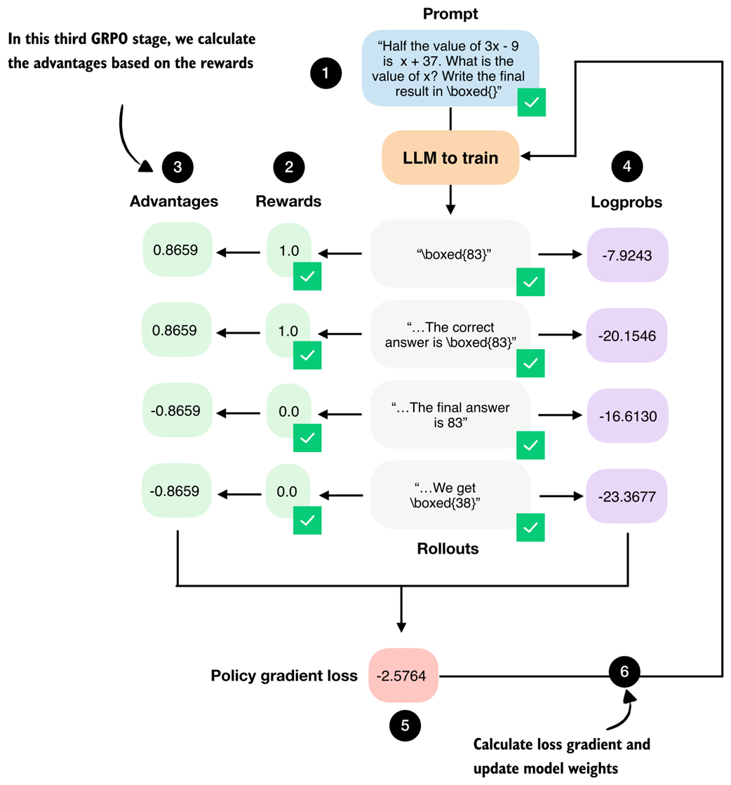 Figure 6.15 The third GRPO stage computes the advantage values from the answer (rollout) correctness rewards.
The advantage values shown in figure 6.15 are computed by a simple formula:
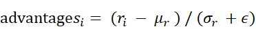
Where $r_i$ denotes the reward of the $i$-th rollout, $\bar{r}$ is the mean reward across the group of rollouts, $\sigma_r$ is the corresponding standard deviation, and $\epsilon$ is a small constant added for numerical stability to avoid zero-division errors.
In code, we can implement the advantage calculation as follows:
Listing 6.8 Calculating advantages
rewards = torch.tensor(rollout_rewards, device=device)
advantages = (rewards - rewards.mean()) / (rewards.std() + 1e-4)
print(rewards)
print(advantages)
The rewards, which we computed in the previous section, are [1., 1., 0., 0.], and the corresponding advantages are [0.8659, 0.8659, -0.8659, -0.8659].
These advantage values capture which responses performed better than average and which performed worse than average within the group.
Note
The “GR” (group relative) in GRPO refers to the fact that GRPO generates multiple answers (rollouts) per prompt, and compares them relative to each other to construct a learning signal.
You might still wonder what the point of converting rewards into advantages is. At a practical level, the advantage values directly scale the gradient during the policy update later.
If the advantage is positive, the gradient increases the likelihood of the actions that produced that rollout. If it is negative, the gradient decreases their likelihood. Rollouts with advantage close to zero contribute very little.
Exercise 6.2: Zero-advantage cases
Modify the rollout rewards so that all rollouts receive the same reward (for example, force all rewards to
0.0or all to1.0). Run the advantage computation and verify that the resulting GRPO loss is zero. Why is this behavior desirable in group-relative policy optimization?
6.12 Scoring rollouts with sequence log-probabilities
We calculated the rewards and advantages from the rewards. Now, we take a separate branch from the rollouts and compute their log-probabilities (logprobs), as shown in figure 6.16. Logprobs measure how likely the model considers each generated token under its current parameters, as discussed in the previous chapter.
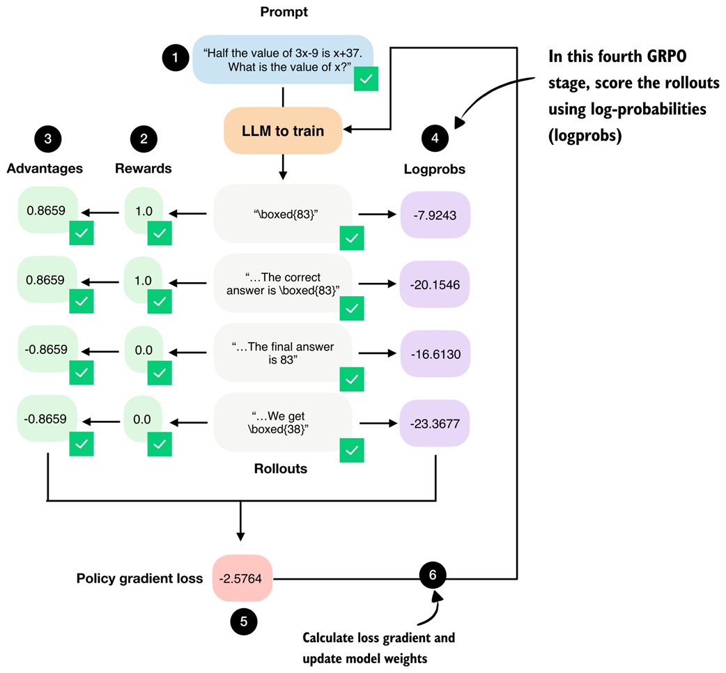 Figure 6.16 The fourth stage in the GRPO pipeline computes log-probabilities for each rollout, which is related to the logprob scorer we developed in the previous chapter.
As shown in figure 6.16, these logprobs, together with the advantages, form the core ingredients of the GRPO policy gradient loss, which we will implement later on.
Coming back to the logprobs, in the previous chapter we implemented an avg_logprob_answer function that computes the per-token logprobs for the model’s answer tokens. These values, often referred to as token-level logprobs in the literature, are obtained by evaluating the likelihood that the model assigns to each generated token under its current parameters.
When averaged across the response, these values are often referred to as token-level logprobs and are commonly used for scoring LLM outputs. Averaging is preferred in this context because it provides length normalization, which makes the scores comparable across responses of different lengths.
Mathematical definition of token-level log-probabilities
Mathematically, the token-level logprobs we computed in the previous chapter can be written as
Here
- $y_1, y_2, …, y_T$ denote the tokens in the generated response of length T
- $y_{<t}$ represents all previously generated tokens
- $x$ is the input prompt
- $W$ denotes the model’s weight parameters.
This expression is mathematically identical to the one used in the previous chapter; we simply switch from $o$ to $y$ to distinguish the generated output tokens from the input prompt for clarity.
For reference, the avg_logprob_answer function from the previous chapter is copied below, which we use to compute the logprobs for the previous prompt and answer_text for illustration purposes.
Listing 6.9 Computing token-level log-probabilities (similar to chapter 5)
@torch.inference_mode()
def avg_logprob_answer(model, tokenizer, prompt, answer, device="cpu"):

    prompt_ids = tokenizer.encode(prompt)
    answer_ids = tokenizer.encode(answer)
    full_ids = torch.tensor(prompt_ids + answer_ids, device=device)

    logits = model(full_ids.unsqueeze(0)).squeeze(0)
    logprobs = torch.log_softmax(logits, dim=-1)

    start = len(prompt_ids) - 1
    end = full_ids.shape[0] - 1

    t_idx = torch.arange(start, end, device=device)
    next_tokens = full_ids[start + 1 : end + 1]
    next_token_logps = logprobs[t_idx, next_tokens]

    return torch.mean(next_token_logps).item()


avg_logprob_val = avg_logprob_answer(
                   model, tokenizer,
                   prompt=prompt,
                   answer=answer_text,
                   device=device)
print(avg_logprob_val)
This returns -0.0615234375.
In GRPO, however, we do not use average token-level logprobs. Instead, we work with sequence-level logprobs.
The reason is that GRPO assigns a single reward and advantage to each rollout, which applies to the entire generated response. Intuitively, logprob should reflect how likely the model was to generate the whole sequence, not an average per token.
We compute sequence-level logprobs by summing the logprobs of all generated tokens. (This sum corresponds to the log-likelihood of producing the full response under the current model parameters.)
In contrast, averaging token-level logprobs normalizes by sequence length. While this normalization is useful for scoring and comparing responses of different lengths, it would unintentionally rescale the learning signal in policy optimization and cause longer and shorter responses to contribute unevenly to the update. (While this is not the intention of the original GRPO formulation, we will revisit token-level logprobs when improving the algorithm in the next chapter.)
We can convert the token-level, length-normalized score into a sequence-level logprobs by dropping the averaging step and replacing torch.mean(next_token_logps) with torch.sum(next_token_logps) in the code in listing 6.9.
The same result can also be obtained by multiplying the averaged logprob by the number of answer tokens, as long as the token count matches exactly:
sequence_logprob_val = avg_logprob_val * (
    len(tokenizer.encode(answer_text))
)
print(sequence_logprob_val)
This now returns -16.2421875.
These sequence-level logprobs scale linearly with the sequence length T, which means that longer responses generally receive more negative logprob values. As a result, for two equally good answers, the optimization implicitly favors the shorter one, since it is cheaper in terms of likelihood. Summed logprobs therefore encourage the model to stop earlier unless producing a longer response is justified by a higher reward.
So, as mentioned before, we can replace torch.mean with torch.sum in the function to obtain sequence-level logprobs. Since the function was run in inference mode in the previous chapter using the @torch.inference_mode() decorator, we need to redefine it (without the decorator) anyway so that PyTorch can track gradients.
In addition, because sample_response from section 6.5 already returns the token_ids and prompt_len, we can simplify the implementation by dropping the explicit tokenization step and the construction of full_ids.
Listing 6.10 Computing sequence-level log-probabilities
def sequence_logprob_draft(model, token_ids, prompt_len):
    logits = model(token_ids.unsqueeze(0)).squeeze(0).float()
    logprobs = torch.log_softmax(logits, dim=-1)

    start = prompt_len - 1
    end = token_ids.shape[0] - 1

    t_idx = torch.arange(start, end, device=token_ids.device)
    next_tokens = token_ids[start + 1 : end + 1]
    next_token_logps = logprobs[t_idx, next_tokens]

    return torch.sum(next_token_logps)

print(sequence_logprob_draft(model, token_ids, prompt_len))
This outputs:
tensor(-16.2998, grad_fn=<SumBackward0>)
First, the result is similar to the -16.2421875 we got earlier (the difference is due to floating-point behavior and rounding).
PyTorch internally builds a computation graph that records each differentiable operation applied to a tensor. The SumBackward0 entry shows that the summation of token log-probabilities is part of this graph, which means gradients can propagate back through the sequence-level log-probability to the model parameters.
This is exactly what we need for policy optimization later, when we implement the training loop to update the model weights via a backward pass. The backward pass applies the backpropagation algorithm, which is the standard method used in deep learning to compute gradients and update neural network weights.
PyTorch computation graphs, gradients, and backpropagation
As the model produces an output, PyTorch records each mathematical operation that leads from the model parameters to that output. This record is called the computation graph. When we later run the backward pass, PyTorch uses this graph to perform backpropagation, that is, computing gradients that describe how changes to the model parameters would affect the final result. If an operation is part of this graph, PyTorch can compute gradients through it during training.
It is not required to understand PyTorch’s computation graphs for this chapter, but interested readers can read more about it in my tutorial at https://sebastianraschka.com/teaching/pytorch-1h/#3-seeing-models-as-computation-graphs.
While this draft implementation is a fully working code implementation, we can simplify it a bit and make it more efficient for GPUs. In particular, we can avoid explicitly constructing index ranges and instead use torch.gather to directly select the logprob corresponding to the generated tokens. Listing 6.11 shows a more compact, optimized version of the same computation that produces identical results while being easier to read and faster to execute.
Listing 6.11 Optimized sequence-level log-probabilities code
def sequence_logprob(model, token_ids, prompt_len):
    logits = model(token_ids.unsqueeze(0)).squeeze(0).float()
    logprobs = torch.log_softmax(logits, dim=-1)
    selected = logprobs[:-1].gather(
        1, token_ids[1:].unsqueeze(-1)
    ).squeeze(-1)
    return torch.sum(selected[prompt_len - 1:])

print(sequence_logprob(model, token_ids, prompt_len))
Similar to the previous code, this returns tensor(-16.2998, grad_fn=<SumBackward0>).
Tip
We could compute these logprobs directly in the
sample_responsefunction to improve efficiency by avoiding callingmodel(...)twice (in both thesample_responseandsequence_logprobfunctions).
Finally, with a robust and efficient sequence-level logprob function in place, we can calculate the respective logprobs of the four different rollouts.
Listing 6.12 Computing sequence-level log-probabilities of all rollouts
rollouts = [
    r"\boxed{83}",
    r"The correct answer is \boxed{83}",
    r"The final answer is 83",
    r"We get \boxed{38}",
]

rollout_logps = []

for text in rollouts:
    token_ids = tokenizer.encode(prompt + " " + text)
    logprob = sequence_logprob(
        model=model,
        token_ids=torch.tensor(token_ids, device=device),
        prompt_len=prompt_len,
    )

    print(f"Answer:  {text}")
    print(f"Logprob: {logprob.item():.4f}\n")

    rollout_logps.append(logprob)
This prints the following:
Answer:  \boxed{83}
Logprob: -7.9243

Answer:  The correct answer is \boxed{83}
Logprob: -20.1546

Answer:  The final answer is 83
Logprob: -16.6130

Answer:  We get \boxed{38}
Logprob: -23.3677
As we can see, shorter and more concise answers receive higher (less negative) sequence-level logprobs than longer or more verbose responses. The exception is the last answer, which receives the lowest score. Note that this is the only answer that contains the incorrect numerical answer value (38 instead of 83), so this also makes intuitive sense.
Overall, this illustrates how summed logprobs naturally favor concise outputs, which is consistent with their role in GRPO when rewards and advantages are applied at the sequence level.
6.13 From advantages to policy updates via the GRPO loss
We now implement the fifth stage of the GRPO pipeline, where the previously computed advantages and log-probabilities are combined into a policy gradient loss. We implement the subsequent weight update (stage six) later as part of the training loop, as shown in figure 6.17.
 Figure 6.17 The fifth stage in the GRPO pipeline computes the policy gradient loss that we use to update the model. Stage number 6, the model weight update, will be implemented as part of the training loop later.
First, we convert the list of the rollout logprobs from the previous section into a PyTorch tensor. Then, we compute the policy gradient loss by multiplying each rollout’s sequence-level logprob by its corresponding advantage, taking the mean across rollouts, and applying a negative sign. Regarding the negative sign, because PyTorch optimizers are defined to minimize a loss, objectives that are naturally written as maximization problems must be sign-flipped.
Listing 6.13 Computing the policy gradient loss
logps = torch.stack(rollout_logps)
pg_loss = -(advantages.detach() * logps).mean()
print(logps)
print(pg_loss)
This prints
tensor([ -7.9243, -20.1546, -16.6130, -23.3677],
grad_fn=<StackBackward0>)
for the logprobs, and the resulting policy gradient loss value is
tensor(-2.5764, grad_fn=<NegBackward0>)
Note that we use .detach() on the advantages because they are treated as fixed learning signals during the policy update. This prevents gradients from flowing back through the advantage computation. This ensures that only the model parameters influencing the logprobs are updated.
For instance, in policy gradient methods, we want to maximize the advantage-weighted logprob of the rollouts, since higher log-probabilities for high-advantage rollouts improve the policy.
So, by multiplying this objective by -1, we convert from the maximization problem into an equivalent minimization problem. Note that minimizing the negative objective produces the exact same parameter updates as maximizing the original one, but this way, it remains compatible with PyTorch’s optimizer implementations.
Maximization versus minimization
To illustrate the sign flipping further with a concrete example, suppose the objective we want to maximize is a simple scalar value $f(x) = 3$.
Under the maximization view, a larger value is better, so 3 is preferable to 2. However, PyTorch optimizers minimize, so they would try to reduce this value, which is the opposite of what we want.
Now, suppose we flip the sign and define the loss as $L(x) = -f(x) = -3$.
Minimizing $L(x)$ is now equivalent to maximizing $f(x)$. For instance, if $L(x)$ decreases from -2 to -3, $f(x)$ increases from 2 to 3.
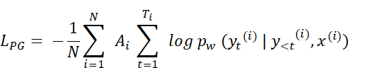
Mathematical definition of the policy gradient loss
For readers who find it easier to follow the computations via mathematical notation, the policy gradient loss used in GRPO can be written as
Here,
- $G$ denotes the number of rollouts,
- $y_1^{(i)}, …, y_{T_i}^{(i)}$ are the tokens of the $i$-th generated response of length $T_i$,
- $y_{<t}^{(i)}$ represents all previously generated tokens in that response,
- $x^{(i)}$ is the corresponding input prompt,
- And $A_i$ is the advantage of the full rollout.
The inner sum computes the sequence-level log-probability of a rollout, while the outer average computes the advantage-weighted log-probabilities across rollouts.
6.14 Putting everything together in a single GRPO function
We have now completed the most challenging parts of this chapter and walked through each GRPO stage in isolation.
Next, we combine the five GRPO stages shown in figure 6.18 into a single compute_grpo_loss function, which we will later use as part of the full training loop.
(Note that here, the term stage refers to a conceptual component of the GRPO loss computation, based on how we walked through the GRPO algorithm step-by-step, not a training step in the outer optimization loop.)
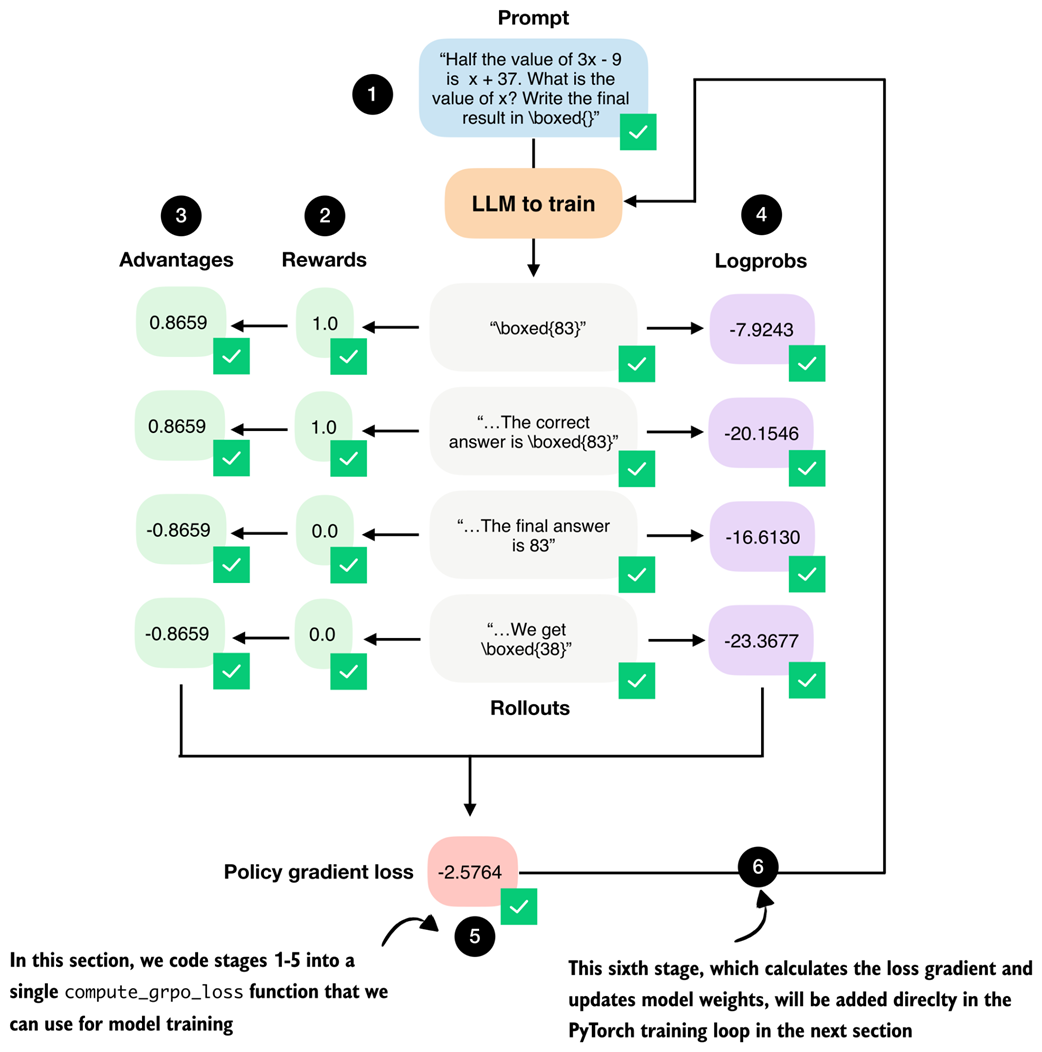 Figure 6.18 Overview of the complete GRPO workflow where (1) multiple rollouts are generated for a prompt, (2) assigned correctness rewards, (3) converted into group-relative advantages, and (4) combined with log probabilities to (5) compute the policy gradient loss. The loss gradients (6) will be computed and used to update the model in the next section.
The compute_grpo_loss function that combines all the stages from figure 6.18 that we discussed previously is shown in listing 6.14 below.
Listing 6.14 Combining all GRPO stages
def compute_grpo_loss(
    model,
    tokenizer,
    example,
    device,
    num_rollouts=2,
    max_new_tokens=256,
    temperature=0.8,
    top_p=0.9,
):
    assert num_rollouts >= 2
    roll_logps, roll_rewards, samples = [], [], []
    prompt = render_prompt(example["problem"])

    was_training = model.training
    model.eval()

    for _ in range(num_rollouts):

        token_ids, prompt_len, text = sample_response(
            model=model,
            tokenizer=tokenizer,
            prompt=prompt,
            device=device,
            max_new_tokens=max_new_tokens,
            temperature=temperature,
            top_p=top_p,
        )

        reward = reward_rlvr(text, example["answer"])

        logp = sequence_logprob(model, token_ids, prompt_len)

        roll_logps.append(logp)
        roll_rewards.append(reward)
        samples.append(
            {
                "text": text,
                "reward": reward,
                "gen_len": token_ids.numel() - prompt_len,
            }
        )

    if was_training:
        model.train()

    rewards = torch.tensor(roll_rewards, device=device)

    advantages = (rewards - rewards.mean()) / (rewards.std() + 1e-4)

    logps = torch.stack(roll_logps)

    pg_loss = -(advantages.detach() * logps).mean()
    loss = pg_loss  # In the next chapter we add a KL term here

    return {
        "loss": loss.item(),
        "pg_loss": pg_loss.item(),
        "rewards": roll_rewards,
        "advantages": advantages.detach().cpu().tolist(),
        "samples": samples,
        "loss_tensor": loss,
    }
The compute_grpo_loss function is relatively self-explanatory as it follows the exact stages we implemented manually in the previous sections. Note, though, that after stage 1, the code proceeds directly to stages 2 and 4, rather than stages 3 and 4. This is purely an implementation choice that simplifies the code structure by avoiding the need for multiple nested for-loops while preserving the same logical sequence of operations.
Also note that the pg_loss (policy gradient loss) is identical to the overall loss in our example. This is because we intentionally omit the KL loss term here and add it later in chapter 7 for completeness. As discussed earlier, GRPO is often reported to perform better on math problems when the KL loss term is omitted, which is why we adopt this simplified objective at this stage.
Next, let’s try the new compute_grpo_loss function on an example from the MATH training dataset to ensure that it works. Here, we sample only a small number of rollouts (num_rollouts=2) and generate a relatively small number of tokens (max_new_tokens=256) for testing purposes. It may still take several seconds until you see the function return the results.
Listing 6.15 Computing GRPO stages on a MATH training example
torch.manual_seed(123)

stats = compute_grpo_loss(
    model=model,
    tokenizer=tokenizer,
    example=math_train[4],
    device=device,
    num_rollouts=2,
    max_new_tokens=256,
    temperature=0.8,
    top_p=0.9
)

pprint(stats)
The output is as follows:
{'advantages': [0.0, 0.0],
 'loss': -0.0,
 'loss_tensor': tensor(-0., grad_fn=<NegBackward0>),
 'pg_loss': -0.0,
 'rewards': [0.0, 0.0],
 'samples': [{'gen_len': 3, 'reward': 0.0, 'text': ' 14'},
             {'gen_len': 256,
              'reward': 0.0,
              'text': ' 4\n'
                      'To solve the problem, let's break it down step by step'
                      '...'}]}
As we can see from the 'rewards' and 'text' entries in the 'samples' field, the model answers incorrectly. As discussed earlier in section 6.4, a correct answer must include \boxed{6}. Since this condition is not met, the reward is zero, which in turn yields zero advantages and a zero loss. In this case, if we were training the model, the gradient would be zero and the model parameters would not be updated.
6.15 Implementing the GRPO training loop
We now have all the necessary components in place to implement the full GRPO training loop. In this final section of the chapter, we bring everything together to train the model via reinforcement learning with verifiable rewards using the GRPO algorithm, as illustrated in figure 6.19.
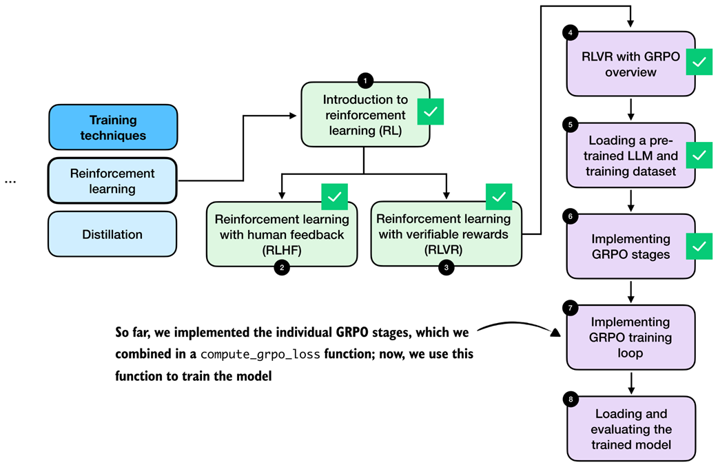 Figure 6.19 After implementing the individual GRPO stages, we now implement the surrounding training loop to update the model weights.
The training loop consists of eight main stages, as shown in figure 6.20. Most of these stages are standard components of a typical PyTorch training loop used for deep neural networks, including LLMs. The only stage specific to reasoning models is stage 4, where we compute the GRPO loss rather than a standard classification loss used in many other types of deep neural networks and LLM pre-training.
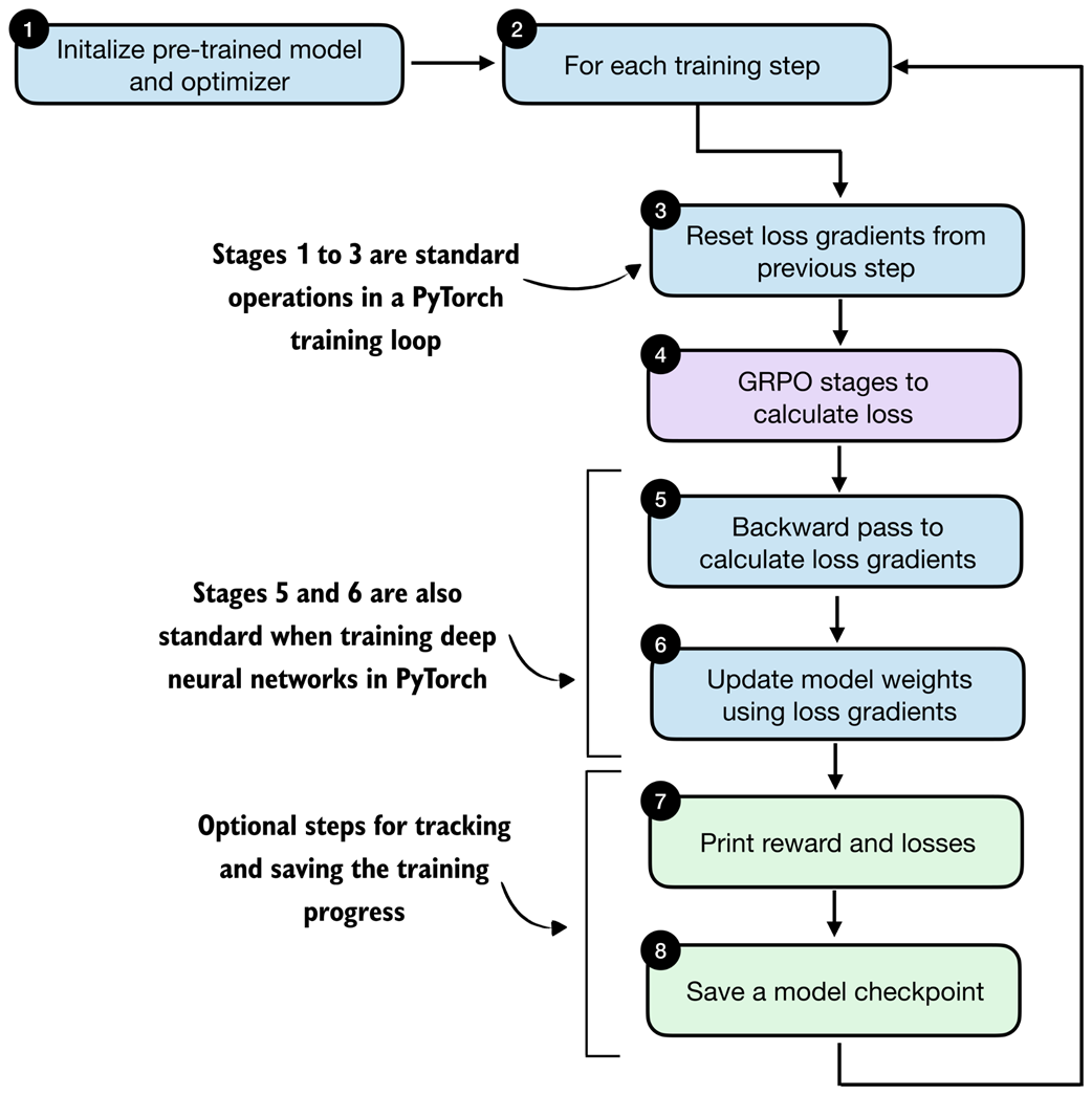 Figure 6.20 Outline of the training loop. The overall structure follows a standard deep learning training loop. The key difference lies in how the loss is computed: instead of a standard supervised objective, the loss is obtained via the GRPO stages (stage 4).
Before discussing the eight stages one by one, it is helpful to first see how they are implemented in code. Listing 6.16 shows the full training loop corresponding to the eight stages illustrated in figure 6.20.
Listing 6.16 Implementing the RLVR training loop
import time

def train_rlvr_grpo(
    model,
    tokenizer,
    math_data,
    device,
    steps=None,
    num_rollouts=2,
    max_new_tokens=256,
    temperature=0.8,
    top_p=0.9,
    lr=1e-5,
    checkpoint_every=50,
    checkpoint_dir=".",
    csv_log_path=None,

):
    if steps is None:
        steps = len(math_data)


    optimizer = torch.optim.AdamW(model.parameters(), lr=lr)
    model.train()
    current_step = 0

    if csv_log_path is None:
        timestamp = time.strftime("%Y%m%d_%H%M%S")
        csv_log_path = f"train_rlvr_grpo_metrics_{timestamp}.csv"
    csv_log_path = Path(csv_log_path)

    try:

        for step in range(steps):


            optimizer.zero_grad()

            current_step = step + 1
            example = math_data[step % len(math_data)]


            stats = compute_grpo_loss(
                model=model,
                tokenizer=tokenizer,
                example=example,
                device=device,
                num_rollouts=num_rollouts,
                max_new_tokens=max_new_tokens,
                temperature=temperature,
                top_p=top_p,
            )


            stats["loss_tensor"].backward()


            torch.nn.utils.clip_grad_norm_(model.parameters(), 1.0)


            optimizer.step()


            reward_avg = torch.tensor(stats["rewards"]).mean().item()
            step_tokens = sum(
                sample["gen_len"] for sample in stats["samples"]
            )
            avg_response_len = (
                step_tokens / len(stats["samples"]) if stats["samples"] else 0.0
            )
            append_csv_metrics(
                csv_log_path, current_step, steps,
                stats["loss"], reward_avg, avg_response_len,
            )
            print(
                f"[Step {current_step}/{steps}] "
                f"loss={stats['loss']:.4f} "
                f"reward_avg={reward_avg:.3f} "
                f"avg_resp_len={avg_response_len:.1f}"
            )


            if checkpoint_every and current_step % checkpoint_every == 0:
                ckpt_path = save_checkpoint(
                    model=model,
                    checkpoint_dir=checkpoint_dir,
                    step=current_step,
                )
                print(f"Saved checkpoint to {ckpt_path}")


    except KeyboardInterrupt:
        ckpt_path = save_checkpoint(
            model=model,
            checkpoint_dir=checkpoint_dir,
            step=max(1, current_step),
            suffix="interrupt",
        )
        print(f"\nKeyboardInterrupt. Saved checkpoint to {ckpt_path}")
        return model

    return model


def save_checkpoint(model, checkpoint_dir, step, suffix=""):
    checkpoint_dir = Path(checkpoint_dir)
    checkpoint_dir.mkdir(parents=True, exist_ok=True)
    suffix = f"-{suffix}" if suffix else ""
    ckpt_path = (
        checkpoint_dir /
        f"qwen3-0.6B-rlvr-grpo-step{step:05d}{suffix}.pth"
    )
    torch.save(model.state_dict(), ckpt_path)
    return ckpt_path


def append_csv_metrics(
    csv_log_path, step_idx, total_steps,
    loss, reward_avg, avg_response_len,
):
    if not csv_log_path.exists():
        csv_log_path.write_text(
            "step,total_steps,loss,reward_avg,avg_response_len\n",
            encoding="utf-8",
        )
    with csv_log_path.open("a", encoding="utf-8") as f:
        f.write(
            f"{step_idx},{total_steps},{loss:.6f},{reward_avg:.6f},"
            f"{avg_response_len:.6f}\n"
        )
This function implements the full RLVR training loop using GRPO. As mentioned earlier, with the exception of stage 4 (the GRPO loss computation), the structure mirrors a conventional PyTorch training loop where we reset gradients, backpropagate a loss, optionally clip gradients, update parameters via an optimizer step, log metrics, and periodically save checkpoints.
Tip
For a general introduction to training neural networks in PyTorch, see sections 3–8 of my PyTorch in One Hour: From Tensors to Training Neural Networks on Multiple GPUs article (https://sebastianraschka.com/teaching/pytorch-1h/).
The key difference here, compared to other standard training loops, is how the loss is constructed. Instead of a standard supervised objective (which is used for the majority of neural networks, for example classifiers, but also for LLM pre-training), the training signal is computed via the GRPO algorithm as part of the RLVR procedure.
Note that, next to the logging steps that print results periodically to track progress, we also save the model checkpoint (a snapshot of the model weights) periodically so we can load, evaluate, and use it later, as discussed in the next section.
Let’s now run the code and train the model. Earlier, we hardcoded the PyTorch device to "cpu" so that all intermediate results more closely match those shown in the book, since "mps" and "cuda" devices can introduce small floating-point differences. Training on a CPU is very slow, though.
For convenience, the listing below already includes two lines that automatically select and activate the appropriate device preceding the train_rlvr_grpo() function call. For instance, it will automatically switch to "cuda" or "mps" simply by running the code in the following listing.
Listing 6.17 Training the model
device = get_device()
model.to(device)

torch.manual_seed(0)

train_rlvr_grpo(
    model=model,
    tokenizer=tokenizer,
    math_data=math_train,
    device=device,
    steps=50,
    num_rollouts=4,
    max_new_tokens=512,
    temperature=0.8,
    top_p=0.9,
    lr=1e-5,
    checkpoint_every=5,
    checkpoint_dir=".",
)
Let’s briefly talk about the settings before we inspect the results. The temperature and top_p settings were chosen in a common range that encourages some diversity in the answers but still results in coherent text for this model. Optionally, you can change these settings and see how they affect the results (reasonable and common ranges are 0.7-0.9).
The number of steps is relatively small at 50, even though the dataset contains 12,000 entries. This is purely due to achieving a reasonable runtime for this educational context, and can be increased. Now, though, it is already sufficient for good results.
The learning rate (lr) can be tweaked, but it is in a reasonable range and works well.
The number of rollouts (num_rollouts=4) and allowed tokens (max_new_tokens=512) are relatively small to reduce resource requirements. If you experience out-of-memory errors, you can further reduce these values, for example, by setting num_rollouts=2 and max_new_tokens=64 for testing purposes.
With the current checkpoint_every=5 setting, the model is saved every 5 steps, and one checkpoint requires approximately 1.5 GB of disk space. In practice, in longer runs, I recommend setting this number to 50 or 100. In this context it is purposefully small for testing purposes. Also, note that an additional checkpoint should be created if the training run is manually interrupted, for instance, by interrupting the Jupyter notebook execution via the "Interrupt the kernel" button.
Let’s now take a brief look at the run’s output (where I interrupted the 50-step run at step 7):
Using Apple Silicon GPU (MPS)
[Step 1/50] loss=-0.0000 reward_avg=0.000 avg_resp_len=87.0
[Step 2/50] loss=-0.0000 reward_avg=0.000 avg_resp_len=6.5
[Step 3/50] loss=-0.0000 reward_avg=0.000 avg_resp_len=5.5
[Step 4/50] loss=0.1404 reward_avg=0.250 avg_resp_len=5.5
[Step 5/50] loss=15.0918 reward_avg=0.250 avg_resp_len=108.2
Saved checkpoint to qwen3-0.6B-rlvr-grpo-step00005.pth

KeyboardInterrupt. Saved checkpoint to qwen3-0.6B-rlvr-grpo-step00006-interrupt.pth
We can see that both the loss and reward values fluctuate, which is normal in RL training.
Note that we print the average reward, which indicates the proportion of sampled responses that are correct. For example, with our num_rollouts=4 setting, a reward_avg of 0.5 means that 2 of our 4 rollouts received a positive reward. Similarly, values of 0.25 and 0.0 indicate one or zero correct responses, respectively.
The loss values themselves should not be over-interpreted. Steps with reward_avg=0.000 produce a near-zero loss because all rollouts receive the same reward, resulting in vanishing group-relative advantages and little to no gradient signal. Larger loss magnitudes, such as at step 3, simply reflect bigger relative differences between rollouts and are typical for GRPO-style objectives, especially at the beginning of training.
Ideally, we want to see two main trends over time:
- The average reward should increase when averaged over many steps, since the model learns to produce more accurate responses.
- The reasoning accuracy should improve (we evaluate this in the next section).
The supplementary materials contain a slightly more sophisticated script version that also contains an option to evaluate the model periodically on subsets of the MATH-500 test dataset to see if the model is improving on the target task: https://github.com/rasbt/reasoning-from-scratch/tree/main/ch06/02_rlvr_grpo_scripts_intro
Batched training
Reinforcement learning can be relatively resource-intensive due to the fact that we have to generate multiple (long) rollouts via the LLMs for each training step. For this reason, the implementation does not support batching.
If you have access to multiple GPUs you can use the optional version of this code with batch and multi-GPU support that can be found in the supplementary materials at https://github.com/rasbt/reasoning-from-scratch/tree/main/ch06/02_rlvr_grpo_scripts_intro, which trains the model faster.
6.16 Loading and evaluating saved model checkpoints
In this final section, as illustrated in figure 6.21, we discuss how to load the saved checkpoints from the RLVR training run of the previous section and how to evaluate the model on the MATH-500 dataset.
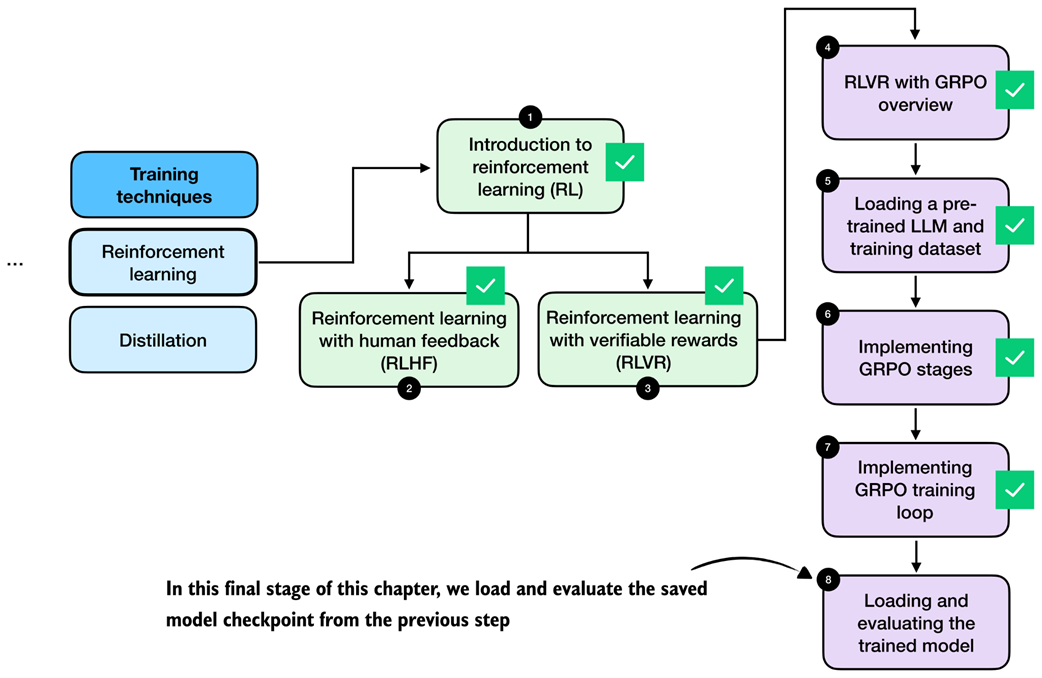 Figure 6.21 The final step of this chapter discusses how we can load the saved model checkpoints and evaluate them.
The saved checkpoints can be loaded using the PyTorch state dict approach, as described in chapter 2, where load_optm points to the corresponding .pth checkpoint file:
model.load_state_dict(torch.load("qwen3-0.6B-rlvr-grpo-step00050.pth"))
Downloading RLVR checkpoints
If you prefer not to run the GRPO training loop locally due to its runtime cost, you can instead download pre-trained checkpoints that I have uploaded. These checkpoints can be fetched either manually or directly from Python using the provided helper function below, which downloads the selected checkpoint and makes it available for evaluation or further experimentation:
from reasoning_from_scratch.qwen3 import download_qwen3_grpo_checkpoints
download_qwen3_grpo_checkpoints(grpo_type="no_kl", step="00050")
Note that this checkpoint was created with similar settings as listing 6.17 except that
num_rollouts=4was increased tonum_rollouts=8.
These checkpoints are fully compatible with the model evaluation utilities introduced in chapter 3, which allows us to evaluate RL-trained models using the same MATH-500 verification pipeline.
For convenience, you can reuse the evaluation scripts provided in the chapter 3 bonus materials (https://github.com/rasbt/reasoning-from-scratch/blob/main/ch03/02_math500-verifier-scripts/evaluate_math500.py) to run evaluations on the MATH-500 dataset by specifying the desired checkpoint path.
For example, to evaluate the qwen3-0.6B-rlvr-grpo-step00050.pth checkpoint file you can run the aforementioned script as
uv run evaluate_math500.py \
--dataset_size 500 \
--which_model base \
--checkpoint_path "qwen3-0.6B-rlvr-grpo-step00050.pth"
(If you are not a uv user, replace uv run with python.)
Table 6.1 compares the original base and reasoning models (rows 1 and 2) to the base model we trained via GRPO in this chapter (rows 3 and 4).
Table 6.1 MATH-500 task accuracy for different base and reasoning models
| Method | Step | Max tokens | Num rollouts | Accuracy | Average tokens | |
|---|---|---|---|---|---|---|
| 1 | Base model (chapter 3) | - | - | - | 15.2% | 78.85 |
| 2 | Reasoning model (chapter 3) | - | - | - | 48.2% | 1369.79 |
| 3 | GRPO (this chapter) | 50 | 256 | 4 | 43.2% | 560.22 |
| 4 | GRPO (this chapter) | 50 | 512 | 4 | 45.6% | 579.81 |
| 5 | GRPO (this chapter) | 50 | 512 | 8 | 47.4% | 586.11 |
The accuracy column in table 6.1 refers to the accuracy on the full 500-sample MATH-500 dataset we used in chapter 3. Note that the “Max tokens” column corresponds to the number of tokens that were allowed per rollout during training. If the number is 512, this encourages the LLM to provide the final boxed answer within this 512 token limit because otherwise it will not receive a reward during training.
The evaluation code was executed with a maximum token limit of 2048, allowing the LLM to generate longer responses during evaluation. The “Average tokens” column averages the response length during the evaluation on the MATH-500 dataset. What we can see is that, compared to the reference reasoning model (row 2), our GRPO models generate shorter responses on average, as expected due to the token-length restriction during training.
Note that the DeepSeek-R1 team observed that responses grew longer over the course of training as the model begins to write intermediate (chain-of-thought) explanations. So, to maximize accuracy, it makes sense not to restrict token length too aggressively during training. However, longer token lengths, especially when coupled with multiple rollouts, require more computational resources, which is why we capped them at a lower limit in this chapter.
As shown in table 6.1, training the reasoning model via GRPO results in 47.4% accuracy (row 5), which is close to the accuracy of the official Qwen3 0.6B reasoning model on MATH-500.
The model’s accuracy could be further improved by increasing the response length, sampling more rollouts per prompt, and training for additional steps. The next chapter introduces practical tips and techniques for monitoring and improving GRPO training outcomes.
We trained the model for only 50 steps, which already appears sufficient to unlock reasoning behavior in the base model. In my experiments, training for longer does not necessarily improve performance and can even reduce accuracy, since the original GRPO formulation can be unstable over longer runs. We address this issue with common GRPO improvements in the next chapter.
Interested readers can find and download additional checkpoints in the range from 50 to 9000 from https://huggingface.co/rasbt/qwen3-from-scratch-grpo-checkpoints/tree/main/grpo_original_no_kl
6.17 Summary
- Reinforcement learning (RL) can be used to train LLMs on human preference labels and verifiable rewards.
- RL is typically applied as post-training on top of a pre-trained base model, and it can be inserted at different stages of an LLM pipeline, including reasoning training and preference tuning.
- RL with human feedback (RLHF) optimizes for human preferences via a two-stage setup: train a reward model from ranked responses, then use reward scores to update the LLM.
- RL with verifiable rewards (RLVR) simplifies RLHF by replacing learned reward models with deterministic, automatically computed verifiers (for example, math answer checking)
- We focussed on RLVR for math reasoning.
- We used GRPO as the policy optimization algorithm that turns verifier rewards into parameter updates; because GRPO directly optimizes the model using sequence-level rewards without requiring a separate value model, it is particularly convenient.
- GRPO is a more resource-friendly alternative to other RL algorithms for LLMs because it avoids training a separate value model and instead derives learning signals from comparisons within a group of sampled rollouts.
- A “rollout” refers to a full model answer (completion) for a prompt; rewards, advantages, and log-probabilities are computed from the rollout in later steps.
- Rewards are computed from a verifier that only grants a reward if the final answer is both correct and extractable in a required format like
"\boxed{}". - Raw rewards are transformed into advantages by normalizing each rollout reward relative to the group mean and standard deviation.
- GRPO also relies on sequence-level log-probabilities, which are computed by summing token log-probabilities over the generated answer tokens.
- Sequence log-probabilities, together with the advantages, form the core policy-gradient objective in GRPO.
- The full GRPO loss computation is combined into a single function that performs rollout sampling, reward computation, advantage calculation, log-prob computation, and policy-gradient loss calculation.
- The surrounding training loop is a standard deep learning loop, with the key difference being that the loss comes from GRPO rather than conventional classification losses.
- Training is resource-intensive because each step requires generating multiple, potentially long rollouts, but even short GRPO runs can increase MATH-500 accuracy from 15% to 47%.